Introduction

This article is for readers who want to use machine learning on Tellus for the first time, but are having a hard time figuring out where to start.

By reading this article, you will learn first hand how to add labels to images that contain the object you want to detect (this time we are using golf courses), then how to use PyTorch to create a learning model to teach a satellite that doesn’t know that object yet how to detect them. We will end by testing our method on Tellus to see if we can get it to detect our desired object.

In this article, we’ll be using the touchvision library to make PyTorch images easier to work with and ImageFolder to easily add labels to them, and will also introduce methods to use learned models via transition learning which will both shorten the process and increase its accuracy.

Although the method we use does make the machine learning process faster, using a CPU for machine learning to understand images still takes a very long time, so the code introduced in this article is intended for only GPU use. To follow along, please use Google Colab or a similar service.
*Satellite images acquired and predicted on Tellus are done so on the Tellus development environment via a CPU.

■This article is for the following kind of person
– Has programming experience, and has performed machine learning before
– Has a certain level of understanding of how neural networks learn and predict (ability to write code not necessary)

The code and image data used in this article are available on github.

(1) Detecting Whether or Not a Golf Course Is Picked up by the Satellite Training Data

Training Data

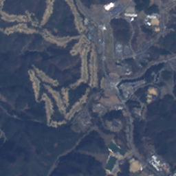
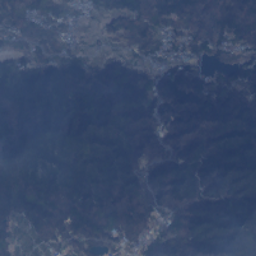
We have prepared images (size 256 x 256) from the prefectures of Chiba and Hyogo that both include (positive) and exclude (negative) golf courses. A simple detection can be done accurately with 100 pictures for each sample.

Please note that Tellus also has restrictions on downloading files locally.

An Example of the Data

An Example of How to Organize Folders

It’s important to organize the folders a certain way when adding labels, so use the following example as a guide.

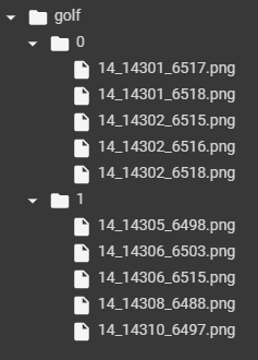
We have set them up like this: 0Folder (Pictures without golf courses), 1Folder (pictures containing golf courses).
*The process actually requires a much larger amount of folders.

This time we will be running a binary expression that determines where there is or isn’t a golf course shown in the picture, but you can also name folders after finding objects (golf, school, etc) to create labels for multiple different categories.

The Code and Its Explanation

As we touched upon earlier, the code and image data used in this article are available on github.

Model Building and Learning (Using a GPU)

The Library Used

Let’s pull up the library we will be using to work with PyToch’s library and images.

import numpy as np
from tqdm import tqdm
from PIL import Image

import torch.nn as nn
from torch.autograd import Variable
import torch

import torchvision.transforms as transforms
import torchvision.models as models
import torchvision

Load the images

By using ImageFolder,  labels will be added automatically to the images in the folders we have set up above. This removes the hassle of creating label data manually by using a data mainframe, or similar software.

Transforming makes it possible to process all of the data while you load it.

It also performs augmentation (a process of increasing the amount of data), when there isn’t enough data available.

transform = transforms.Compose(
            [
            # 画像サイズが異る場合は利用して画像サイズを揃える
            # transforms.Resize((256,256)),
             
            # 左右対称の画像を生成してデータ量を増やす(Augmentation)
             transforms.RandomHorizontalFlip(),

            # PyTorchで利用するTensorの形式にデータを変換
             transforms.ToTensor()   
             ])

# google colab等で実行する際にフォルダ内に .ipynb_checkpoints があると、ラベルの対象になるので削除
!rm -rf golf/.ipynb_checkpoints

# ImageFolder を利用して読み込む
data = torchvision.datasets.ImageFolder(root='./golf', transform=transform)

Use the code below

data.class_to_idx
実行結果> {'0': 0, '1': 1}

And if you get results like this, it means your images have been labeled correctly.

Separating the Data for Training and Validation

The image data is split up into training data and validation data. By using random_split, it will split up the data randomly to a specified ratio.

train_size = int(0.8 * len(data))
validation_size  = len(data) - train_size
data_size  = {"train":train_size, "validation":validation_size}

data_train, data_validation = torch.utils.data.random_split(data, [train_size, validation_size])

train_loader = torch.utils.data.DataLoader(data_train, batch_size=16, shuffle=True)
validation_loader = torch.utils.data.DataLoader(data_validation, batch_size=16, shuffle=False)

dataloaders  = {"train":train_loader, "validation":validation_loader}

Model Creation

For the task of image recognition, we’ll use a learning model which uses resnet18 for its ability to accurately predict objects.

model = models.resnet18(pretrained=True)
model

By running the above code, it should display the following network configuration model.

ResNet(
  (conv1): Conv2d(3, 64, kernel_size=(7, 7), stride=(2, 2), padding=(3, 3), bias=False)
  (bn1): BatchNorm2d(64, eps=1e-05, momentum=0.1, affine=True, track_running_stats=True)

・・・
(中略)
・・・

  (avgpool): AdaptiveAvgPool2d(output_size=(1, 1))
  (fc): Linear(in_features=512, out_features=1000, bias=True)
)

If you run it the way it is, the output for the last layer (out_features) is set as 1000 and needs to be changed to 2 in order to get the desired results of 0 or 1. Also, for the learned model, fix the combined parts that have already been learned in order for the machine to learn only the final output layer.

*Be aware that having the machine learn the entire network may cause over-learning.

# 現在のモデルすべてのパラメータの requires_grad を False にすることで
# ネットワークの重みを固定することができる
for parameter in model.parameters():
    parameter.requires_grad = False

# 今回は0,1の予測のため、最終的な出力を2個に設定
model.fc = nn.Linear(512, 2)

# CPU環境の場合は不要
model = model.cuda()

Model Learning

Now we’ll have it learn from the model we created.
It trains and validates for each epoch.
The loss function uses cross entropy.

lr = 1e-4
epoch = 50
optim = torch.optim.Adam(model.parameters(), lr=lr, weight_decay=1e-4)

# CPU環境の場合は cuda() は不要
criterion = nn.CrossEntropyLoss().cuda()

def train_model(model, criterion, optimizer, num_epochs):
    for epoch in tqdm(range(num_epochs)):
        epoch_loss = 0
        epoch_acc = 0

        for phase in ['train', 'validation']:
            if phase == 'train':
                model.train()
            else:
                model.eval()

            current_loss = 0.0
            current_corrects = 0

            for data in dataloaders[phase]:
                inputs, labels = data

                # CPU環境では不要
                inputs = inputs.cuda()
                labels = labels.cuda()

                outputs = model(inputs)

                _, preds = torch.max(outputs.data, 1)

                loss = criterion(outputs, labels)

                if phase == 'train':
                    optimizer.zero_grad()
                    loss.backward()
                    optimizer.step()

                # CPU環境では item() 不要
                current_loss += loss.item() * inputs.size(0) 
                current_corrects += torch.sum(preds == labels)

            epoch_loss = current_loss / data_size[phase]

            # CPU環境では item() 不要
            epoch_acc = current_corrects.item() / data_size[phase]

            print('{} Loss: {:.4f} Acc: {:.4f}'.format(phase, epoch_loss, epoch_acc))

    return model

trained_model = train_model(model, criterion, optim, epoch)

The log shows the loss and accuracy (acc) rates for the training and validation data, so make sure that as it learns, the loss rate decreases for validation, while its acc rate increases. If the acc reaches 100%, there is a chance it may have over-learned.

Model File Output

Save the learned model to a file and upload it to the Tellus development environment.

torch.save(trained_model.state_dict(), './golf-model.pth')

Prediction

Now we will run the model against the data we used to learn to make predictions and see if it has learned correctly or not. Take an image from the learning data folder and save them as train-positive.png and train-negative.png. The accuracy should be higher since we are using the same images we used at the learning stage.

Set it to validation mode, and load the test image to run it through the model.

trained_model.eval()
imsize = 256
loader = transforms.Compose([transforms.Scale(imsize), transforms.ToTensor()])

def image_loader(image_name):
    image = Image.open(image_name).convert("RGB")
    image = loader(image)
    image = Variable(image, requires_grad=True)
    image = image.unsqueeze(0)  
    # CPU環境の場合は cuda() は不要
    return image.cuda()
m = nn.Softmax(dim=1)

Let’s take a look at the predictions made by the network for both train-positive.png and train-negative.png.

image = image_loader('./train-positive.png')
print(m(model(image)))
実行結果> tensor([[0.2003, 0.7997]], device='cuda:0', grad_fn=)

image = image_loader('./train-negative.png')
print(m(model(image)))

実行結果> tensor([[0.7765, 0.2235]], device='cuda:0', grad_fn=)

The results will be shown as [possibly negative, possibly positive] between 0 and 1. This is how it looks, with train-positive.png on the right and train-negative.png on the left, and with the right having larger numbers, showing it made accurate predictions.

(2) Acquiring the Picture on Tellus and Making a Prediction (Using a CPU)

Now let’s try using new data that hasn’t been tested yet to see whether or not our model can make accurate predictions.

We used Chiba and Hyogo as examples used for the training data. As I am from Hanno City in Saitama, where there are a few golf courses, I thought it would be a good place to test our model. Let’s find the data on Tellus, then download it onto the Tellus development environment to see whether or not it can make accurate predictions.

How to Search for and Acquire Data on Tellus

The data we learned about this time was for golf courses, but when running it against untested data, our results weren’t so great.

Taking a look at the two different sets of data, it looks like the data we used for learning was taken during the winter. Though there was no snow in the images, the grass on the golf courses happened to be dead. The new data set appears to have been taken in the summer, with nice green grass.

It looks like this is something we will have to look out for when conducting machine learning. We may need to have it learn from pictures taken for each of the seasons in order to get more accurate results.

With that, I’ll explain how to acquire satellite images from specific daes on Tellus OS.
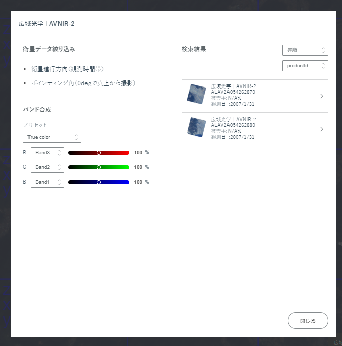
First, choose the satellite you want data from on the left, then click the upper-right hand grid icon, and apply the tile data.

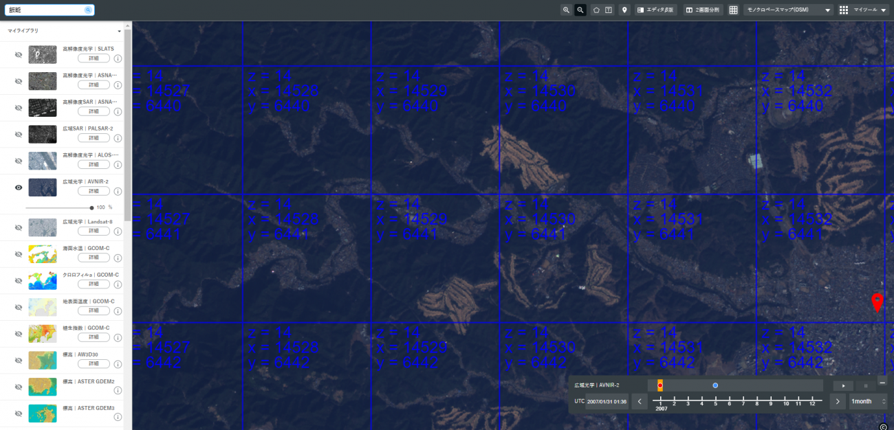
This time, we’ll set the negative as (x=14528, y=6441, z=14), and the positive as the neighboring tile at (x=14529, y=6441, z=14) to try and get our image data.

But wait, if you keep using API to acquire　 “https://gisapi.tellusxdp.com/blend/{z}/{x}/{y}.png”, it will acquire the latest satellite data, so if you want data from the satellite you’ve selected in the bar in the lower right-hand portion of the screen, you will need to go to the menu on the left and click the “details” button on your desired satellite (we’re using AVNIR-2 this time).

If you do that, it should show you the screen below, where you will choose from the satellite shown.

Then it should show you even more in-depth information on the satellite image. Use the path where it says tile_path to select a specific time and date for the satellite image you want.

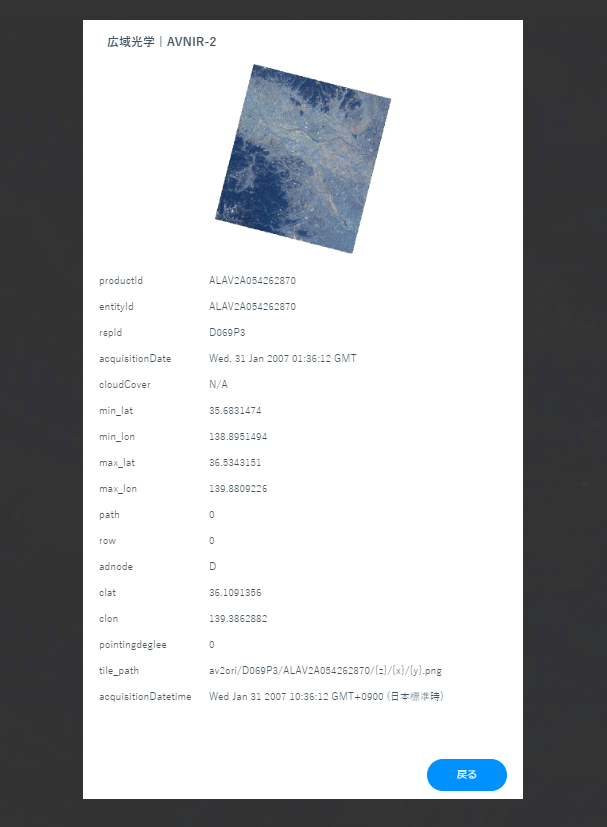
Now it knows where to get the image you desire, let’s try loading it onto the Tellus development platform.
Also be sure to upload the golf-model.pth we created earlier through machine learning.

The Library Used

The library hasn’t changed much, though there are more acquired images and display libraries.

import torchvision.transforms as transforms
import torchvision.models as models

import torch.nn as nn
import torch
from torch.autograd import Variable

import requests

from PIL import Image
from io import BytesIO
import matplotlib.pyplot as plt

%matplotlib inline

Acquire the Image

Set the token, and define the method that can acquire the images from the path you selected earlier.

TOKEN = 'YOUR-TOKEN'
def get_image(rspid, productid, z, x, y):
    url = f"https://gisapi.tellusxdp.com/blend/av2ori/{rspid}/{productid}/{z}/{x}/{y}.png"
    headers = {
        'Authorization': 'Bearer ' + TOKEN
    }
    r = requests.get(url, headers=headers)
    return Image.open(BytesIO(r.content))

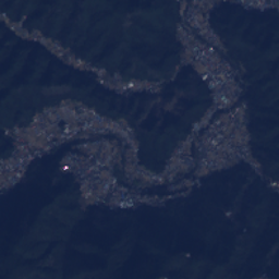
Start by first downloading and displaying the positive data that contains golf courses, and save them as “test-positive.png”.

im_array = get_image('D069P3', 'ALAV2A054262870', 14, 14529, 6441)
plt.imshow(im_array)
im_array.save('test-positive.png')

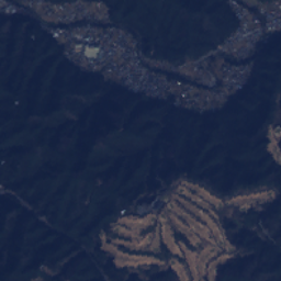
Next, for the neighbouring tile which doesn’t contain any golf courses, save it as “test-negative.png”.

im_array = get_image('D069P3', 'ALAV2A054262870', 14, 14528, 6441)
plt.imshow(im_array)
im_array.save('test-negative.png')

Load the Model

Just like we did locally, download resnet18, then enter the network data of the uploaded model after aligning it with the output. We’ll specify the map_location since we’re using data we learned with a GPU on a CPU.

model = models.resnet18(pretrained=True)
model.fc = nn.Linear(512, 2)
model.load_state_dict(torch.load('./golf-model.pth', map_location=torch.device('cpu')))

Loading the Images

Just like we did when predicting locally, convert the data into images and run it against the model.

model.eval()

imsize = 256
loader = transforms.Compose([transforms.Scale(imsize), transforms.ToTensor()])

def image_loader(image_name):
    image = Image.open(image_name).convert("RGB")
    image = loader(image)
    image = Variable(image, requires_grad=True)
    image = image.unsqueeze(0)
    return image

m = nn.Softmax(dim=1)

Predicting

Load the images you acquired before and have the system make its prediction.

image = image_loader('./test-positive.png')
m(model(image))

実行結果> tensor([[0.0111, 0.9889]], grad_fn=)

The numbers on the right are higher, which means there is a high chance that the images contain a golf course.

image = image_loader('./test-negative.png')
m(model(image))

実行結果> tensor([[0.8987, 0.1013]], grad_fn=)

The numbers on the left are higher, which means there is a low chance that the images contain a golf course.

It looks like our model was successful in determining whether or not the pictures have golf courses in them.

You can use the same process to detect things like buildings (such as mega-solar power plants), so try it out for yourself.

(3) Introducing Tellus' User Community

I’d like to end this with an introduction of our Discord group.

The writer of this article, Mr. Ueda, will be in charge of running a community that supplements Tellus’ official support by holding regular study groups, facilitating collaborations between users, and acting as a place for users to ask for help when they get stuck.

We currently hold a weekly “mob programming” event on our Discord where we have multiple programmers work together to write a specific code. The code introduced in this article for finding golf courses was created during one of our mob programming events.

This is a great place for people who are interested in using Tellus but don’t know where to start to learn about satellite data, so feel free to join our free Discord server!

Discord Server Invite Link