Tellus has released a function to distribute original data from the satellite data provider in addition to the tiled data that can be easily checked with Tellus OS (on the browser).
For further information, please read this article.

Original data is a difficult thing to handle without knowledge of satellite data, but if you know how to use it, the range of what you can do will expand dramatically.

This article describes how to extract and visualize complex images (images with phase and reflection intensity information of radio waves) from PALSAR-2 L1.1 data released on Tellus in accordance with the format called the CEOS format.

■What is PALSAR-2 processing level L1.1?

L1.1 is a high-resolution complex image

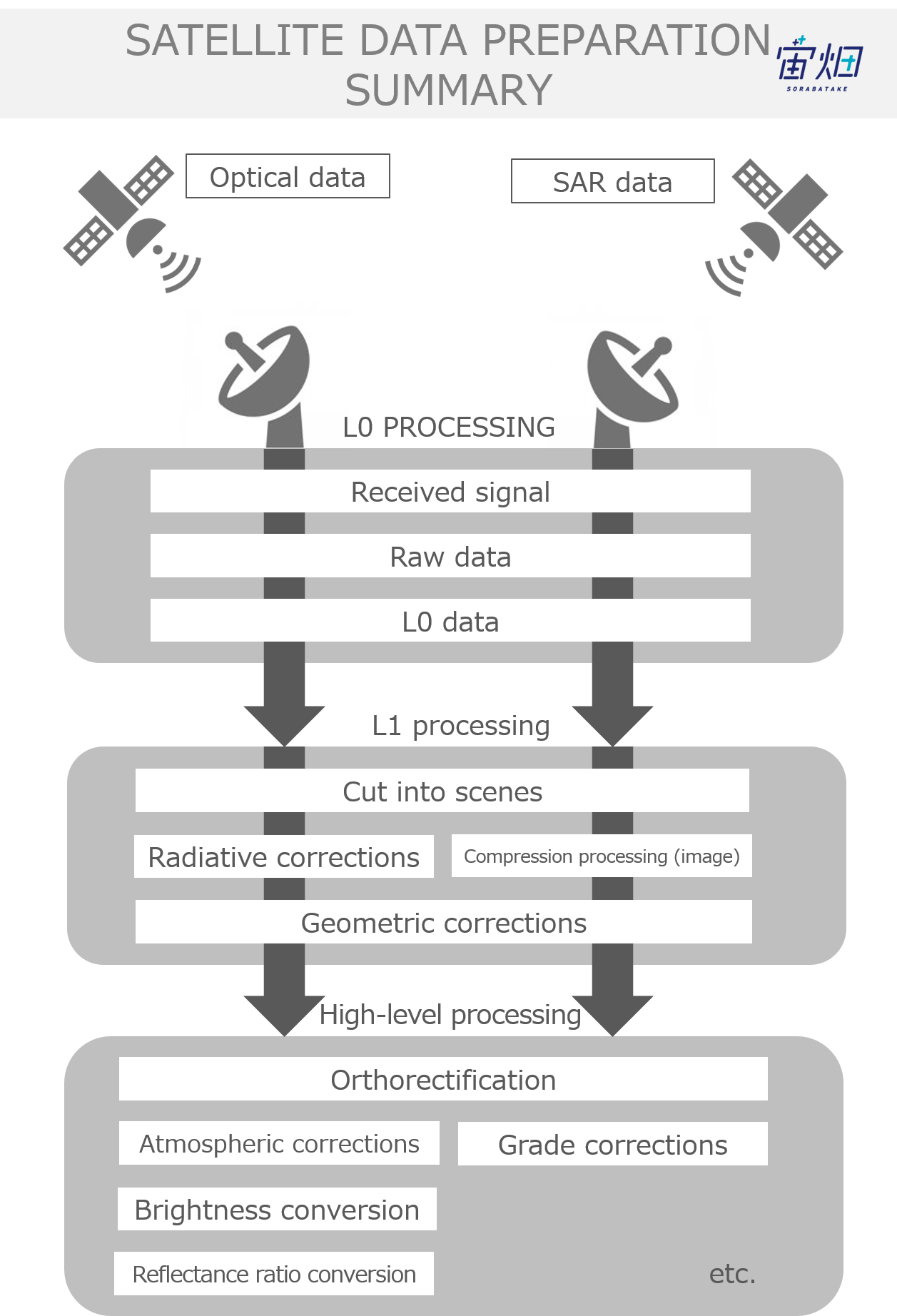
There are several processing levels for SAR images. L1.1 is the data immediately after imaging, and is the base product for subsequent processing. It is sometimes called SLC (Single Look Complex) and is a complex image with the highest resolution.

It has radio wave phase information

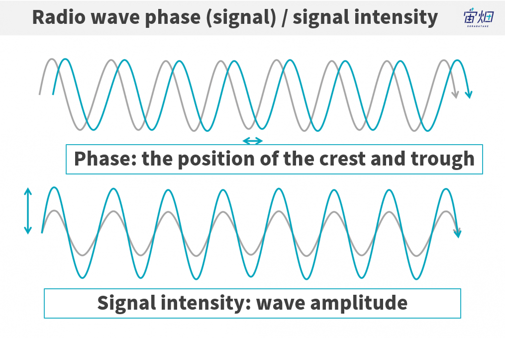
A major feature is that it retains not only the intensity of the reflected radio wave but also the phase information of the radio wave emitted by SAR (information on the angle from -180 ° to + 180 °), so by superimposing images taken at different times, we can measure geomorphic change.

Other processing levels of PALSAR-2

Other PALSAR-2 processing levels are as follows.

-L1.0: the data before imaging and it requires advanced expertise to image
-L1.5: The vertical and horizontal resolution of the image has been corrected by multi-look processing. However, at this point, the phase information is lost.
-L2.1: The image is orthorectified using the existing digital elevation model (DEM). From this processing level it can be treated in the same way as general optical images.

See below for details.

■Get PALSAR-2 L1.1 data

See Tellusの開発環境でAPI引っ張ってみた (Use Tellus API from the development environment) for how to use the development environment (JupyterLab) on Tellus.

Acquire product ID

This time, as we download the product acquired from the satellite as it is, first of all, specify the desired location and time and create a program that acquires the product ID.

First of all, use the following code to specify the desired latitude and longitude, and acquire the product ID. The sample is Kasumigaura in Ibaraki Prefecture.

--Sample code⓪--

import os, requests

TOKEN = "自分のAPIトークンを入れてください"

def search_palsar2_l11(params={}, next_url=''):
    if len(next_url) > 0:
        url = next_url
    else:
        url = 'https://file.tellusxdp.com/api/v1/origin/search/palsar2-l11'
    headers = {
        "Authorization": "Bearer " + TOKEN
    }
    
    r = requests.get(url,params=params, headers=headers)
    if not r.status_code == requests.codes.ok:
        r.raise_for_status()
    return r.json()

def main():
    ret = search_palsar2_l11({'after':'2019-1-01T15:00:00'})
    lat = 36.046
    lon = 140.346
    for i in ret['items']:
        lon_min = i['bbox'][0]
        lat_min = i['bbox'][1]
        lon_max = i['bbox'][2]
        lat_max = i['bbox'][3]
        if lat > lat_min and lat < lat_max and lon > lon_min and lon < lon_max:
            print(i['dataset_id'])    
if __name__=="__main__":
       main()

Download data set

After obtaining the product ID, download all the data sets included in the product with the following code.

--Sample code①--

import os, requests
 
TOKEN = "自分のAPIトークンを入れてください"

def publish_palsar2_l11(dataset_id):
    url = 'https://file.tellusxdp.com/api/v1/origin/publish/palsar2-l11/{}'.format(dataset_id)
    headers = {
        "Authorization": "Bearer " + TOKEN
    }
    r = requests.get(url, headers=headers)
    if not r.status_code == requests.codes.ok:
        r.raise_for_status()
    return r.json()
def download_file(url, dir, name):
    headers = {
        "Authorization": "Bearer " + TOKEN
    }
    r = requests.get(url, headers=headers, stream=True)
    if not r.status_code == requests.codes.ok:
        r.raise_for_status()
    if os.path.exists(dir) == False:
        os.makedirs(dir)
    with open(os.path.join(dir,name), "wb") as f:
        for chunk in r.iter_content(chunk_size=1024):
            f.write(chunk)
def main():
    dataset_id = 'ALOS2249732860-190107'
    print(dataset_id)
    published = publish_palsar2_l11(dataset_id)
    for file in published['files']:
        file_name = file['file_name']
        file_url = file['url']
        print(file_name)
        file = download_file(file_url, dataset_id, file_name)
    print('done')
if __name__=="__main__":
    main()

Data set contents

By executing the above, a directory with the same name as the scene ID is created in the current directory on Jupyter, and the file is stored in that directory. With this, the download of L1.1 data is completed. The contents of the folder are as follows.

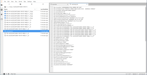
To briefly explain the contents of this dataset,

-Image data with the extension .jpg
This is a thumbnail image to easily check satellite data.  Since the satellite data itself is of large data capacity and it takes time to check content, the resolution is reduced at the time of imaging.

-IMG-AA-XXXXXX.tif (the file which starts with IMG)
The image data we will handle this time is this file.
The character string in the AA part indicates the type of image data.

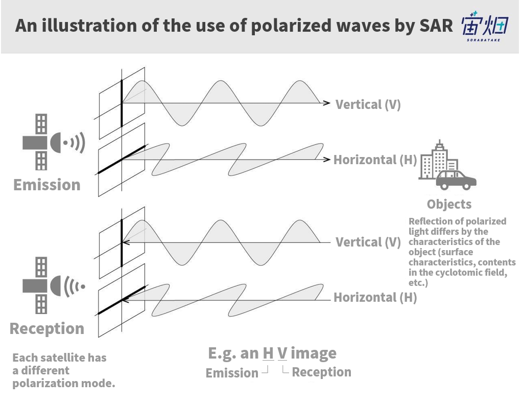
There are four types of data (HH, HV, VH, VV) in total, categorized by the type of transmission/reception radio waves called polarization. They indicate whether it is a vertical polarization (V) or a horizontal polarization (H) with respect to transmission (1st letter) and reception (2nd letter) respectively.

As shown in the figure above, the products, of which there are four types in total, are generally called full polarimetry.

This time, I want to process HH image data.

Other files store information needed to process images. I will refer to these files as appropriate during the process.

■This is the hard part! Decoding CEOS format

Now, let’s process the image data.

Some would say, well, although you could call it processing, like other optical images, don’t we just get an array of two-dimensional images?

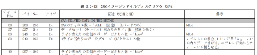
As explained in the previous article ([How to Use Tellus from Scratch] Obtain Original Data of Provider), SAR data is stored in the specified position for each byte according to the CEOS format, so you need to get all the information you need by yourself.

The PALSAR-2 product format is available here.

For example, it is written as follows.

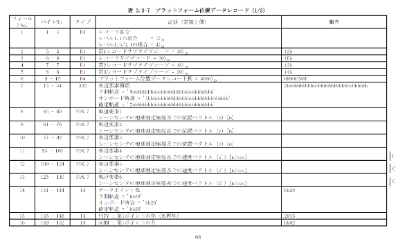
Many people must have given up on processing raw data after seeing this product format. ． ． This time, we will focus on extracting SAR image data and explain it with sample code!

Open binary file

First, open the binary file containing the image data.

dataset_id = 'ALOS2249732860-190107'
fp = open(os.path.join(dataset_id,'IMG-HH-ALOS2249732860-190107-HBQL1.1__D'),mode='rb')

How to handle binary files

Next, we will explain how to handle binary files. Python uses seek () to move the pointer to the specified position. For example, take the vertical and horizontal sizes of the image from the following locations in the product format.

fp.seek(236)
nline = int(fp.read(8))
print(nline)
fp.seek(248)
npixel = int(fp.read(8))
print(npixel)

Extract SAR data

Lastly, once you know the size of the image, extract the SAR data. The following SAR RAW SGINAL DATA is the corresponding part of the format.

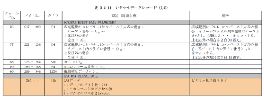
To be honest, this is not easy, so here is a simple illustration to help us how to understand it.

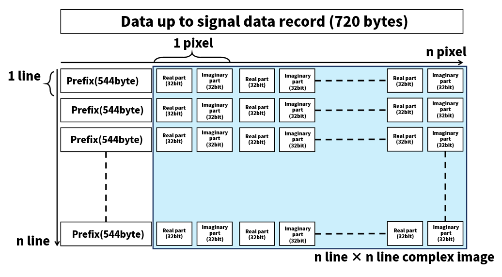
The script to capture all the complex image data according to this figure is as follows.

nrec = 544 + npixel*8
fp.seek(720)
data = struct.unpack(">%s"%(int((nrec*nline)/4))+"f",fp.read(int(nrec*nline)))
# シグナルデータを32bit浮動小数点数として読み込み
data = np.array(data).reshape(-1,int(nrec/4)) # 2次元データへ変換
data = data[:,int(544/4):int(nrec/4)] # prefixを削除
slc = data[:,::2] + 1j*data[:,1::2]

nrec = 544 + npixel*8
fp.seek(720)
data = struct.unpack(">%s"%(int((nrec*nline)/4))+"f",fp.read(int(nrec*nline)))
# シグナルデータを32bit浮動小数点数として読み込み
data = np.array(data).reshape(-1,int(nrec/4)) # 2次元データへ変換
data = data[:,int(544/4):int(nrec/4)] # prefixを削除
slc = data[:,::2] + 1j*data[:,1::2]

In the above code, one entire scene of the product is processed, so the memory size may be insufficient and the operation may stop in certain development environments. In that case, please limit the line and pixel range in advance as shown in the script below.

import os
import numpy as np
import struct
 
def main():
    dataset_id = 'ALOS2249732860-190107'
    fp = open(os.path.join(dataset_id,'IMG-HH-ALOS2249732860-190107-HBQL1.1__D'),mode='rb')

    col = 2000
    row = 2000
    cr = np.array([3000,3000+col,8000,8000+row],dtype="i4");

    fp.seek(236)
    nline = int(fp.read(8))
    fp.seek(248)
    ncell = int(fp.read(8))
    nrec = 544 + ncell*8

    nline = cr[3]-cr[2]
    fp.seek(720)
    fp.read(int((nrec/4)*(cr[2])*4))
    data = struct.unpack(">%s"%(int((nrec*nline)/4))+"f",fp.read(int(nrec*nline)))
    data = np.array(data).reshape(-1,int(nrec/4))
    data = data[:,int(544/4):int(nrec/4)]
    slc = data[:,::2] + 1j*data[:,1::2]
    slc = slc[:,cr[0]:cr[1]]
    print(slc)

if __name__=="__main__":
    main()

This completes the complex image.

■Decompose a complex image into phase and intensity

Once a complex image is obtained, decompose the complex number stored in each pixel into the phase and intensity components. The sample code is as follows.

Numpy has a handy feature that makes the conversion easy.

The intensity is logarithmically converted according to the calibration formula (https://www.eorc.jaxa.jp/ALOS-2/calval/calval_jindex.htm). On the other hand, the phase is converted to [-π to π] by this operation.

sigma = 20*np.log10(abs(slc)) -83.0 -32.0
phase = np.angle(slc)

Now, let’s make an image by using the following procedure.

■Visualize ① intensity image

The result of visualizing the intensity image is as follows. Here, histogram equalization is also corrected because some pixels have strong or weak reflection intensities.

import cv2
import matplotlib.pyplot as plt

sigma = np.array(255*(sigma-np.amin(sigma))/(np.amax(sigma)-np.amin(sigma)),dtype="uint8")
sigma = cv2.equalizeHist(sigma)
plt.figure()
plt.imshow(sigma, cmap = "gray")
plt.imsave('figure.jpg', sigma, cmap = "gray")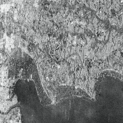

The intensity image literally shows the intensity of the reflected radio waves.

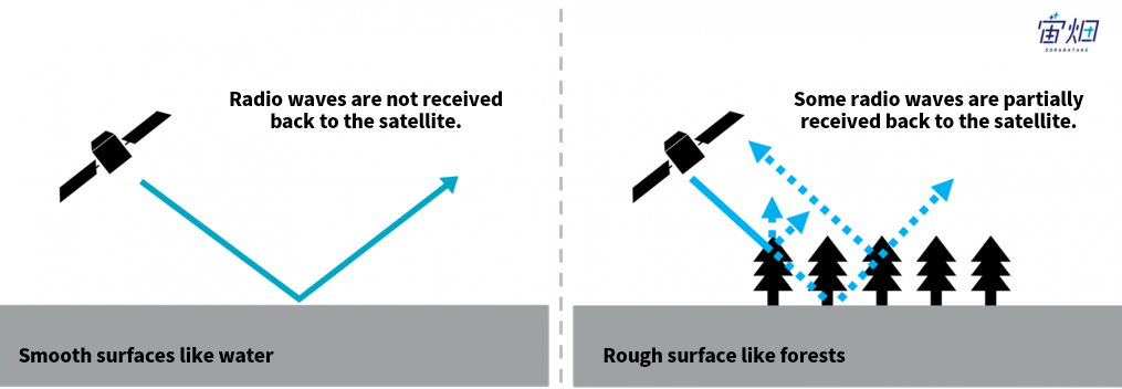
It is a strong signal received back when the object is something like metal that reflects radio waves fully, whilst as waves penetrate through trees etc., reflections from the ground beneath trees are also reflected back  Also, the sea or lakes look black as water does not reflect radio waves well.

When you check the image, you can see landscapes such as mountains and fields, arterial roads and large buildings, but the visibility is not as good as with optical images. Actually, intensity images are typically combined with optical images in order to extract more information. On the other hand, the benefit of a SAR image is that unlike optical images, they provide an image independent of how the sunlight shines on objects.

(For more detail,  please refer to “The basics of Synthetic Aperture Radar (SAR) Use Cases, Obtainable Information, Sensors, Satellites, Wavelengths.)

■ Visualize ② phase image

The result of visualizing the phase image is as follows.

phase = np.array(255*(phase - np.amin(phase))/(np.amax(phase) - np.amin(phase)),dtype="uint8")
plt.figure()
plt.imshow(phase, cmap = "jet")
plt.imsave('phase.jpg', phase, cmap = "jet")

It looks like the image of random noise. To begin with, I will briefly explain what a phase image is.

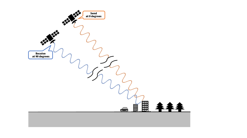
As shown above, when the SAR signal is transmitted by satellite, reflects on the object, and  is received, the phase of each pixel indicates at what degree the last wave was at. (At this time, since the satellite is also moving, the position at transmission and at reception differ.) The center frequency of PALSAR-2 is about 1.2GHz and the wavelength is about 23cm. Since the resolution on the ground is merely 3m or so, the phase information is buried in one pixel.

Even if the resolution is very high, there could be an error in the positioning accuracy of the satellite at the time of observation, or that the phase may shift due to the ionosphere. So, we are afraid we cannot extract information on the landscape when it is reflected only from the phase information obtained in a single observation. In order to make effective use of phase information, it is necessary to compare it with the data acquired at a different time at the same point in strict alignment. This is commonly called “interference analysis.”

Although it was generally considered that interference analysis requires advanced processing technology, the Remote Sensing Technology Center (RESTEC) provides an interference analysis result called RISE in the Tellus market released on February 27. 。 Sorabatake will introduce examples of interference analysis in future articles, so please look forward to seeing them.

* In actuality, the SAR signal does not continuously emit such a carrier wave as shown in the figure but transmits a frequency-modulated pulse signal at regular intervals, so consider the figure as a conceptual diagram to understand what a phase is. As it happens, the pulse signal itself also undergoes a Doppler shift by the relative movement speed between the satellite and the ground, and the amount of the shift is used to determine from which position on the ground surface the radio wave is reflected. By applying this to all pulse signals, we can reproduce the received signal as if it were received by a huge, stationary antenna. This is the mechanism of “synthetic aperture”, but I will not go into further details now.

Among the interference analyses using SAR phase information, “differential interference SAR” is well known. It extracts changes over time on the ground. It is described in detail in the previous article.
https://sorabatake.jp/4343/

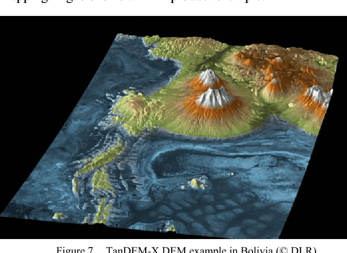
A Digital Elevation Model (DEM) can also be created by using phase information.  This is a technology to observe SAR simultaneously with two satellites and uses the parallax effect by the distance between the satellites to view the ground surface stereoscopically. By this, we can frequently update maps with high accuracy, and apply this technology to grasp the scale of disasters by capturing three-dimensional changes in terrain like landslides and avalanches, and to also view and then manage the amount of embankment at construction sites etc., is being studied as well.

Summary

In this article, I have described how to handle the CEOS format unique to satellite data.
Processing original data from a SAR provider requires knowledge specific to satellite data, but I hope now we know for sure that anyone can do it if one knows the basics.
And by deepening your understanding of original data from satellites, the greater the value of satellite data becomes.
Next time, I intend to visualize land cover using a PALSAR-2 L2.1 full polarimetric image.