Using Tellus to Determine Land Subsidence via InSAR Analysis [Code Included]
This article will go over coding algorithms for the interferometric analysis of SAR images. Anyone can use this code to create their own InSAR images.
Are all of our readers making good use of standard data from PALSAR-2 (the synthetic aperture radar built into ALOS-2 developed by JAXA) released on Tellus? We will introduce how it has been used up until now in this article.
Imaging PALSAR-2 L1.1 using Tellus [with code]
Tellus Takes on the Challenge of Calculating Land Coverage Using L2.1 Processing Data from PALSAR-2
This article will go over coding algorithms of SAR images for an interferometric analysis. Anyone can use this code to create their own InSAR images.
Working with Interferometric SAR requires a high level of skill, which has created a standard for it to be done with a specialized, for-profit software, the inner workings of which are a black box. This makes it difficult for entry-level analysts to use this technology, and creates a challenge when trying to expand its use. We are hoping that this article can help overcome this challenge.
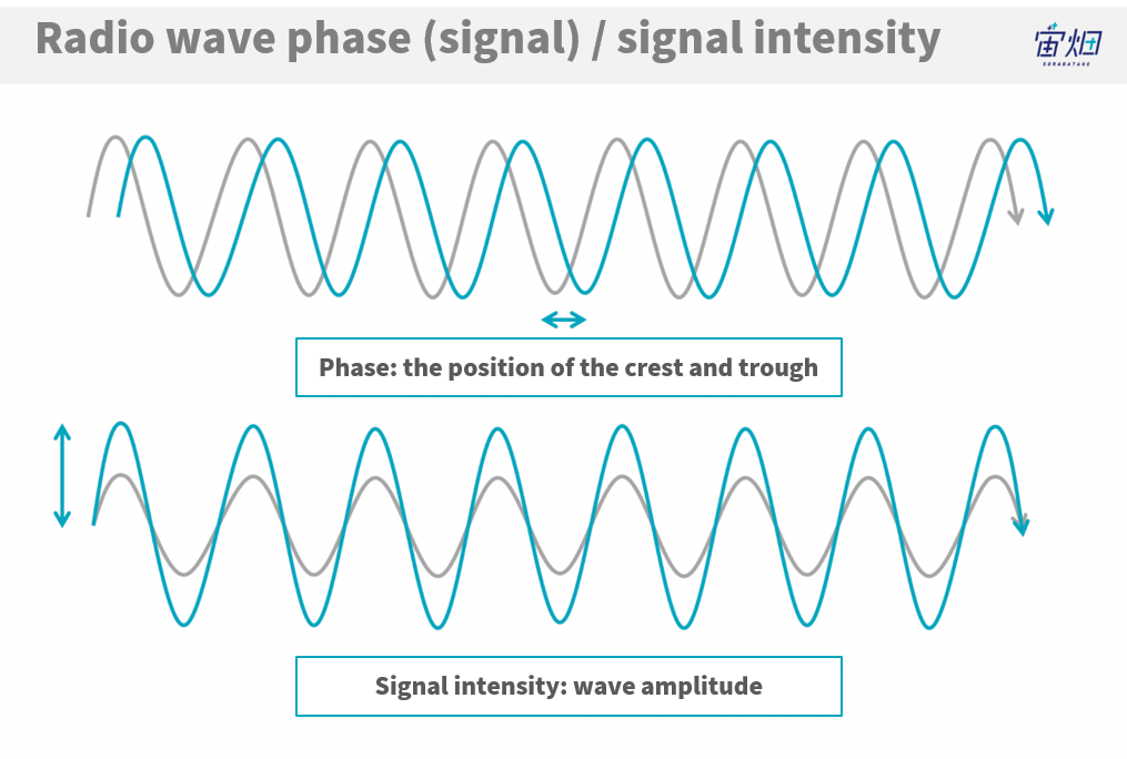
What is InSAR?
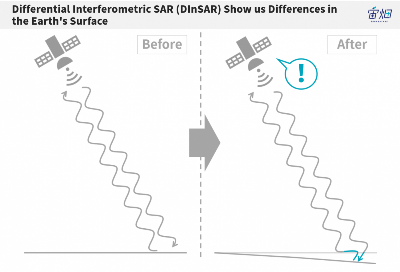
InSAR could be considered a technology that finds changes in the earth’s surface by measuring the phase contrast in waves. When a satellite emits waves from a fixed position, it can detect shifts in the phases of waves reflected back at it which signify changes in the earth’s surface which may occur over a span of time.
Find out more about InSAR in this published article, explained by the Remote Sensing Society of Japan (RESTEC).
This article will focus on programming this using the Tellus development environment.
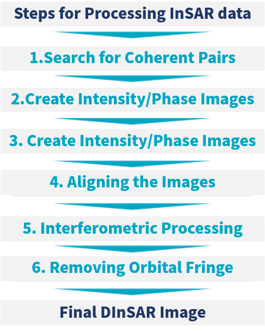
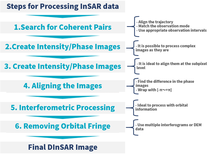
The steps for processing InSAR data is as follows. We will explain each step.
(1) Finding a Coherent Pair
There are a few hurdles when it comes to actually utilizing InSAR data. The first hurdle is finding a pair of coherent images (a coherent pair). Two pictures of the same part of the earth doesn’t necessarily make them coherent.
The three primary conditions for checking the coherence of images are as follows.
1. The images were taken from the same trajectory (position, direction).
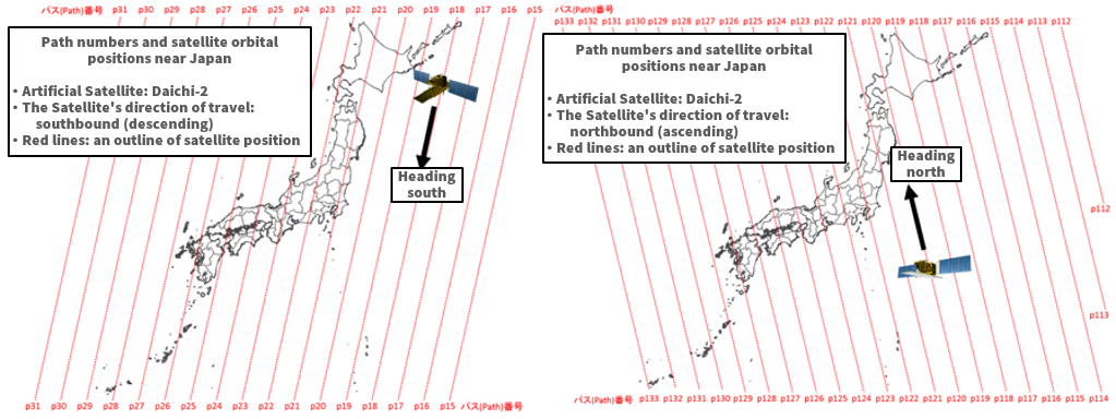
(Left: The trajectory moving from north to south. Right: The trajectory moving from south to north.) Credit : Geospatial Information Authority of Japan Source : https://insarmap.gsi.go.jp/mechanism/orbit_observation_region.html
There is a chance that the position from which a satellite captured an image may be different. If the images have been taken from different positions, this naturally changes the way they look, and makes them incoherent. It is vital that the images be taken from the same spot. You must check the number that has been assigned to each satellite, which signifies the trajectory it follows, which is called its “path”.
Furthermore, satellites orbit the earth from north to south (descending) and from south to north (ascending), so it is important to match the direction of its path as well.
2.They need to be taken in the same observation mode
Just like how a smart phone has a panorama and hi-def mode, SAR sensors have different observation modes for different purposes, each with varying resolutions and observation ranges.
The PALSAR-2 images we used for this article can be divided into the three types of observation modes below.
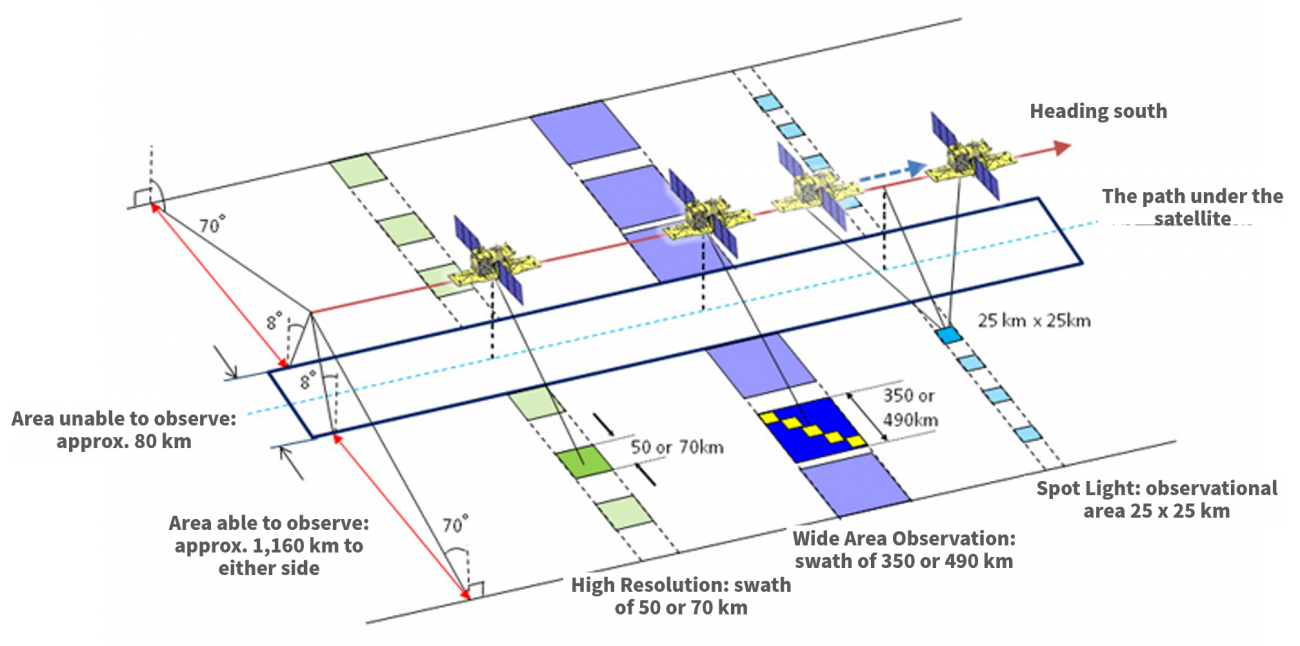
◆ Spotlight Mode
Recreates the most detailed observation images with a resolution of 1 m x 3 m (with an observation area of 25 km)
◆High Resolution Mode
Can choose a resolution between 3 m, 6 m, and 10 m (with an observation area of 50 or 70 km)
◆Wide Area Observation Mode
Is able to observe a wide area in one image (with a resolution between 60 to 100 m, and an observation area of 350 km or 490 km)
It is important to make sure that the observation modes match when searching for a Coherent Pair.
3.Making sure there isn’t too much time between observations
If too much time has passed between observations, there may be other changes in addition to movement in the earth surface itself, such as changes in vegetation, which increase factors to take into account for an accurate analysis. Most analyses are made in intervals of a couple of months.
So let’s try finding a pair using the conditions above.
We should also mention that this article will use a theme park built on reclaimed land around the Tokyo bay area that was known to be built on flat land that had already had changes to it.
*Please be aware that methods for processing land that has more complex features, such as mountainous areas, requires a more advanced code.
The Search Code for a Product
First we search for the relative product by entering the coordinates of the area we would like to find. When we do this, we must make sure that we are searching for a coherent pair, so we include trajectory information and mode of observation, as in conditions 1. and 2.
The results of our code should give us something like the following:
import requests

TOKEN = "自分のAPIトークンを入れてください"

def search_palsar2_l11(params={}, next_url=''):
    if len(next_url) > 0:
        url = next_url
    else:
        url = 'https://file.tellusxdp.com/api/v1/origin/search/palsar2-l11'
    headers = {
        "Authorization": "Bearer " + TOKEN
    }

    r = requests.get(url,params=params, headers=headers)
    if not r.status_code == requests.codes.ok:
        r.raise_for_status()
    return r.json()

def main():
    lat = 35.630
    lon = 139.882
    for k in range(100):
        if k == 0:
            ret = search_palsar2_l11({'after':'2017-01-01T15:00:00'})
        else:
            ret = search_palsar2_l11(next_url = ret['next'])
        for i in ret['items']:
            lon_min = i['bbox'][0]
            lat_min = i['bbox'][1]
            lon_max = i['bbox'][2]
            lat_max = i['bbox'][3]
            if lat > lat_min and lat  lon_min and lon < lon_max:
                print(i['dataset_id'],i['beam_number'],i['path_number'],i['frame_number'],i['mode'])
        if 'next' not in ret:
            break
if __name__=="__main__":
       main()
The results of our code should give us something like the following:
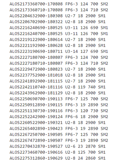
Think of “beam_number”, “path_number”, “frame_number” that we receive as a part of the trajectory data. If these do not match, then typically, they won’t be a coherent pair. The information for the picture located in the center of the Tokyo Bay is registered as beam_number=U2-8, path_number=18, fram_number=2900, so let’s focus our search on these.
| Variable name | Description | Storage example |
| beam_number | The combination of the observation mode and the angle at which the satellite is capturing images. | ex.) F2-4 |
| path_number | The path the satellite follows | 001~207 |
| frame_number | This shows the range of the area captured by the photo and the center of the photo. | 0000~7190 |
Please check JAXA’s homepage for more details.
“Mode” can also be used to show one of ALOS-2’s multiple observation modes, with SM1 being stripmap1 (a resolution of 3 m), and SM2 being SStripmap2 (a resolution of 6 m). We will take this opportunity to use the higher resolution with the SM1 mode for our article.
We will show the script we use for downloading the selected coherent pairs below. (We have left out previously covered functions below)
Please make sure there is enough space on your hard drive (about 30GB) before running the script.
import os
def publish_palsar2_l11(dataset_id):
url = 'https://file.tellusxdp.com/api/v1/origin/publish/palsar2-l11/{}'.format(dataset_id)
headers = {
"Authorization": "Bearer " + TOKEN
}
r = requests.get(url, headers=headers)
if not r.status_code == requests.codes.ok:
r.raise_for_status()
return r.json()
def download_file(url, dir, name):
headers = requests.utils.default_headers()
headers["Authorization"] = "Bearer " + TOKEN
r = requests.get(url, headers=headers, stream=True)
if not r.status_code == requests.codes.ok:
r.raise_for_status()
if os.path.exists(dir) == False:
os.makedirs(dir)
with open(os.path.join(dir,name), "wb") as f:
for chunk in r.iter_content(chunk_size=1024):
f.write(chunk)
def main():
for k in range(100):
if k == 0:
ret = search_palsar2_l11({'after':'2017-01-01T15:00:00'})
else:
ret = search_palsar2_l11(next_url = ret['next'])
for i in ret['items']:
if i['beam_number'] == 'U2-8' and i['path_number'] == 18 and i['frame_number'] == 2900 and i['mode'] == 'SM1':
dataset_id = i['dataset_id']
published = publish_palsar2_l11(dataset_id)
for file in published['files']:
file_name = file['file_name']
file_url = file['url']
print(file_name)
file = download_file(file_url, dataset_id, file_name)
if 'next' not in ret:
break
if __name__=="__main__":
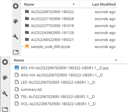
main()There are 5 products related to this example. A file with the same name as the product ID is created in the Current Directory with the data saved within it. It should look something like the example below. This is how you get the data needed for processing InSAR images. We should also note that the data on observation dates, 3/22/18, 3/22/18, 6/28/18, 10/18/18, 11/29/18, 3/21/19, has been taken in intervals of a few months at a time.
The thumbnails for each of the five products can be seen as follows.
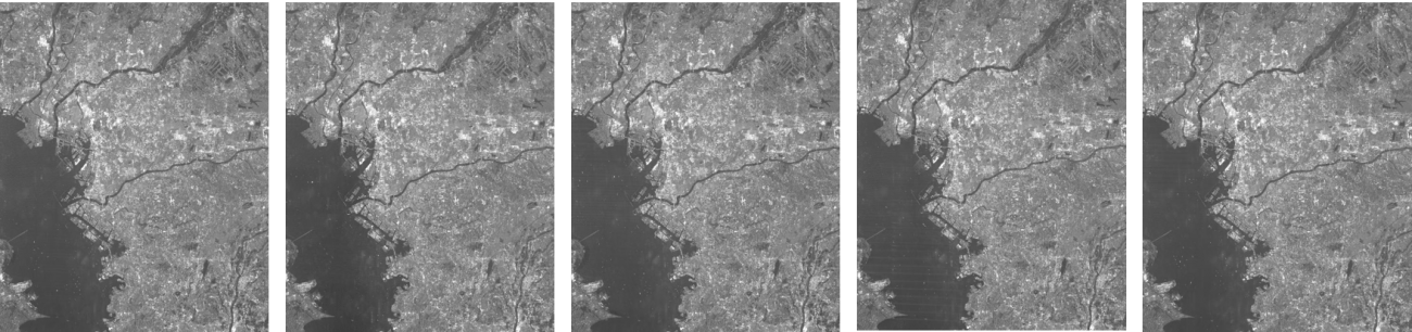
Original data provided by JAXA
Furthermore, the processing level for ALOS-2 is set at L1.1, and this has an impact on the photos. We will fix this in the next step.
(2) Creating Intensity and Phase Images
This has been introduced in a previous article (Imaging PALSAR-2 L1.1 using Tellus [with code]), but due to the nature of SAR images being of electromagnetic waves, the data can be split up into “intensity” and “phase” data. To put it simply, intensity is the “strength at which the waves bounce back” and the phase is the “height and wavelength of the waves”.
We will create an intensity image and a phase image from each of the products. The image is too large, which creates a memory error, so we will specify the longitude and latitude to trim it.
import os
import numpy as np
import struct
import math
import matplotlib.pyplot as plt
from io import BytesIO
import cv2

def gen_img(fp,off_col,col,off_row,row):
    cr = np.array([off_col,off_col+col,off_row,off_row+row],dtype="i4");
    fp.seek(236)
    nline = int(fp.read(8))
    fp.seek(248)
    ncell = int(fp.read(8))
    nrec = 544 + ncell*8

    nline = cr[3]-cr[2]
    fp.seek(720)
    fp.seek(int((nrec/4)*(cr[2])*4))
    data = struct.unpack(">%s"%(int((nrec*nline)/4))+"f",fp.read(int(nrec*nline)))
    data = np.array(data).reshape(-1,int(nrec/4))
    data = data[:,int(544/4):]
    data = data[:,::2] + 1j*data[:,1::2]
    data = data[:,cr[0]:cr[1]]
    sigma = 20*np.log10(abs(data)) - 83.0 - 32.0
    phase = np.angle(data)
    sigma = np.array(255*(sigma - np.amin(sigma))/(np.amax(sigma) - np.amin(sigma)),dtype="uint8")
    sigma = cv2.equalizeHist(sigma)
    return sigma, phase

def get_pl(fp,latlon):
  fp.seek(720+4096+1620+4680+16384+9860+325000+511000+3072+728000+2064,0)
  c = np.zeros(25,dtype="float64")
  for i in range(25):
    c[i] = fp.read(20)
  d = np.zeros(25,dtype="float64")
  for i in range(25):
    d[i] = fp.read(20)
  lat0 = float(fp.read(20))
  lon0 = float(fp.read(20))
  phi = np.zeros(2,dtype="float64")
  lam = np.zeros(2,dtype="float64")
  phi[0] = latlon[0] - lat0
  phi[1] = latlon[1] - lat0
  lam[0] = latlon[2] - lon0
  lam[1] = latlon[3] - lon0
  pl = np.zeros(4,dtype="float64")
  for i in range(5):
    for j in range(5):
      id = i*5+j
      pl[0] += c[id]*lam[0]**(4-j) * phi[0]**(4-i)
      pl[1] += c[id]*lam[1]**(4-j) * phi[1]**(4-i)
      pl[2] += d[id]*lam[0]**(4-j) * phi[0]**(4-i)
      pl[3] += d[id]*lam[1]**(4-j) * phi[1]**(4-i)
  return pl

def main():
    #合計5つのプロダクトに対して同じ処理を行ってください
    ids = ['ALOS2206702900-180322',
           'ALOS2221192900-180628',
           'ALOS2237752900-181018',
           'ALOS2243962900-181129',
           'ALOS2260522900-190321']
    for i, dataset_id in enumerate(ids):
        fpimg = open(os.path.join(dataset_id,'IMG-HH-'+dataset_id+'-UBSR1.1__D'),mode='rb')
        fpled = open(os.path.join(dataset_id,'LED-'+dataset_id+'-UBSR1.1__D'),mode='rb')

        latlon = np.array([35.625, 35.640, 139.86, 139.90],dtype="float64")
        pl = np.array(np.ceil(get_pl(fpled,latlon)),dtype=np.int64)
        print(pl)
        off_col = pl[1]
        col = pl[0] - pl[1]
        off_row = pl[3]
        row = pl[2] - pl[3]
        print(col,row)
        sigma, phase = gen_img(fpimg,off_col,col,off_row,row)
        sigma = np.fliplr(sigma) #左右反転
        phase = np.fliplr(phase) #左右反転
        np.save('sigma0{}.npy'.format(i + 1),sigma) #numpy配列として出力
        np.save('phase0{}.npy'.format(i + 1),phase) #numpy配列として出力
        # 画像の保存
        plt.imsave('sigma0{}.jpg'.format(i + 1), sigma, cmap = "gray")
        plt.imsave('phase0{}.jpg'.format(i + 1), phase, cmap = "jet")

    dataset_id = 'ALOS2206702900-180322'
#    dataset_id = 'ALOS2221192900-180628' #合計5つのプロダクトに対して
#    dataset_id = 'ALOS2237752900-181018' #同じ処理を行ってください。
#    dataset_id = 'ALOS2243962900-181129'
#    dataset_id = 'ALOS2260522900-190321'
    fpimg = open(os.path.join(dataset_id,'IMG-HH-'+dataset_id+'-UBSR1.1__D'),mode='rb')
    fpled = open(os.path.join(dataset_id,'LED-'+dataset_id+'-UBSR1.1__D'),mode='rb')

    latlon = np.array([35.625, 35.640, 139.86, 139.90],dtype="float64")
    pl = np.array(np.ceil(get_pl(fpled,latlon)),dtype=np.int64)
    print(pl)
    off_col = pl[1]
    col = pl[0] - pl[1]
    off_row = pl[3]
    row = pl[2] - pl[3]
    print(col,row)
    sigma, phase = gen_img(fpimg,off_col,col,off_row,row)
    sigma = np.fliplr(sigma) #左右反転
    phase = np.fliplr(phase) #左右反転
    np.save('sigma01.npy',sigma) #numpy配列として出力
    np.save('phase01.npy',phase) #numpy配列として出力
    #np.save('sigma02.npy',sigma) #numpy配列として出力
    #np.save('phase02.npy',phase) #numpy配列として出力
    #np.save('sigma03.npy',sigma) #numpy配列として出力
    #np.save('phase03.npy',phase) #numpy配列として出力
    #np.save('sigma04.npy',sigma) #numpy配列として出力
    #np.save('phase04.npy',phase) #numpy配列として出力
    #np.save('sigma05.npy',sigma) #numpy配列として出力
    #np.save('phase05.npy',phase) #numpy配列として出力
if __name__=="__main__":
       main()
The images we get look like this.
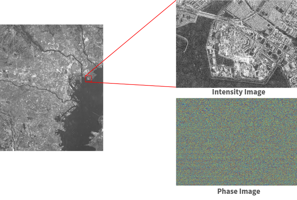
Original data provided by JAXA
Intensity images show the strength with which waves are reflected back at the satellite by calibrating the reflection coefficient into a logarithm. Phase images are shown in a range between -180π – +180π.
With a resolution of 3 m, the level of visibility allows us to differentiate buildings. The phase images, on the other hand, don’t have this kind of visibility.
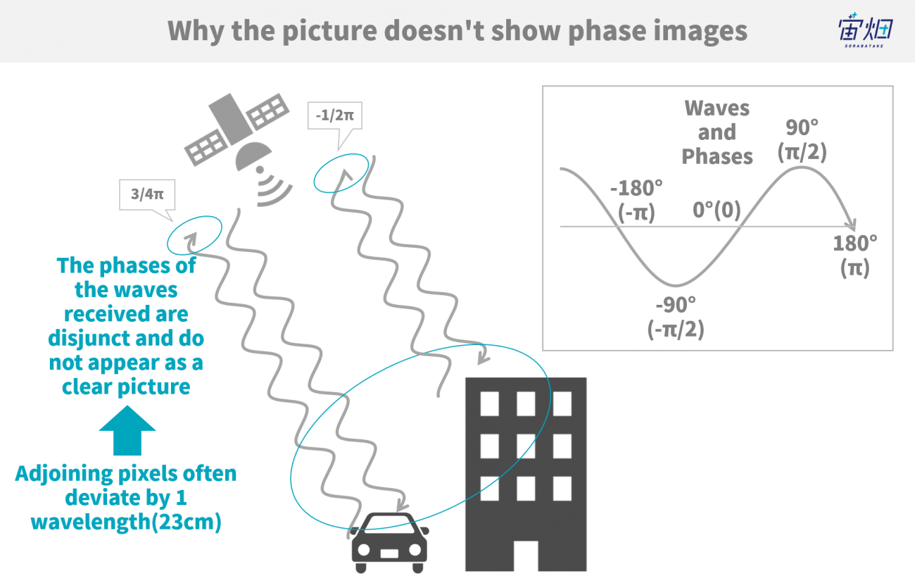
This makes sense seeing as the wavelength of the waves emitted by PALSAR-2 are about 23 cm, and at a resolution of 3 m, and there is ambiguity for each wave between adjoining pixels and that there is almost no correlation between these pixels.
When working with SAR, it is incredibly difficult to make observations with a resolution too large for the wavelength, so as a rule of thumb, there isn’t much use in the phase data gathered from one phase image. That is why it is important for there to be interference.
Using the program above, create a NumPy array for each of the five products’ intensity and phase images. This brings us to our next step, where we conduct our analysis of their interference.
(3) Image Alignment and Interferometric Processing
So most of our readers are probably wondering what the interferometric part of InSAR actually means? What is happening can be broken down in the next two steps.
- 1.Using two intensity images to align the images
- 2.Check the difference between two phase images, and wrap it within phases of [-π~+π]*
*This refers to the process of returning [-π~+π] – [-π~+π] = [-2π~+2π] back to [-π~+π].
The alignment from 1. is particularly important. We are able to get better results by accurately overlapping the two images.
There are lots of methods for aligning images, with the standard method involving the use of intensity images to make alignments at a sub pixel level (below one pixel) and to interpolate the phase images.
However, the interference conducted for this example was done with a very simple algorithm, so we aligned them at one pixel and cut off the parts that don’t match. This is a simple shift which uses a function available in the Open CV library of Tellus environment.
The process for 2. is a simple subtraction. This could be considered the “moment” of interference. On a more general note, regarding the two complex images normally included in the intensity component, one of the complex conjunctions is multiplied on top of the other, which is also considered interferometric processing and it is doing the exact same thing. This article has made it easier for beginners by separating the images into intensity and phase data, so it might be easier to do this by regarding “interferometric processing as finding the difference between phases”.
Also, this example uses five different products, so we will use image number 3 as a reference and the other four images to make our interference.
import os
import numpy as np
import matplotlib.pyplot as plt
import math
from io import BytesIO
import cv2

#画像の位置合わせを行う関数
#強度画像A,Bを用いて変位量を求めて、位相画像C,Dをその変位量で画像をカットします
#変位量は小数点以下まで結果がでますが、それを四捨五入して整数として扱っています
def coregistration(A,B,C,D):
    py = len(A)
    px = len(A[0])
    A = np.float64(A)
    B = np.float64(B)
    d, etc = cv2.phaseCorrelate(B,A)
    dx, dy = d
    print(d) #画像の変位量です
    if dx = 0:
        dx = math.ceil(dx)-1
        dy = math.ceil(dy)
        rD = D[dy:py,0:px+dx]
        rC = C[dy:py,0:px+dx]
    elif dx < 0 and dy = 0 and dy = 0 and dy >= 0:
        dx = math.ceil(dx)
        dy = math.ceil(dy)-1
        rD = D[dy:py,dx:px]
        rC = C[dy:py,dx:px]
    return rC, rD

def wraptopi(x):
    x = x - np.floor(x/(2*np.pi))*2*np.pi - np.pi
    return x

def main():
    #強度画像と位相画像の読み込み。また、ここで画像のサイズを統一しています。
    phase01 = np.load('phase01.npy')[0:1028,0:1420]
    sigma01 = np.load('sigma01.npy')[0:1028,0:1420]
    phase02 = np.load('phase02.npy')[0:1028,0:1420]
    sigma02 = np.load('sigma02.npy')[0:1028,0:1420]
    phase03 = np.load('phase03.npy')[0:1028,0:1420]
    sigma03 = np.load('sigma03.npy')[0:1028,0:1420]
    phase04 = np.load('phase04.npy')[0:1028,0:1420]
    sigma04 = np.load('sigma04.npy')[0:1028,0:1420]
    phase05 = np.load('phase05.npy')[0:1028,0:1420]
    sigma05 = np.load('sigma05.npy')[0:1028,0:1420]

    #プロダクトNo.1とNo.3で干渉処理を実施
    coreg_phase01, coreg_phase03 = coregistration(sigma01,sigma03,phase01,phase03)
    ifgm01 = wraptopi(coreg_phase01 - coreg_phase03)

    #プロダクトNo.2とNo.3で干渉処理を実施
    coreg_phase02, coreg_phase03 = coregistration(sigma02,sigma03,phase02,phase03)
    ifgm02 = wraptopi(coreg_phase02 - coreg_phase03)

    #プロダクトNo.4とNo.3で干渉処理を実施
    coreg_phase04, coreg_phase03 = coregistration(sigma04,sigma03,phase04,phase03)
    ifgm04 = wraptopi(coreg_phase04 - coreg_phase03)

    #プロダクトNo.5とNo.3で干渉処理を実施
    coreg_phase05, coreg_phase03 = coregistration(sigma05,sigma03,phase05,phase03)
    ifgm05 = wraptopi(coreg_phase05 - coreg_phase03)

    np.save('ifgm01.npy',ifgm01)
    np.save('ifgm02.npy',ifgm02)
    np.save('ifgm04.npy',ifgm04)
    np.save('ifgm05.npy',ifgm05)
    #画像の保存
    plt.imsave('ifgm01.jpg', ifgm01, cmap = "jet")
    plt.imsave('ifgm02.jpg', ifgm02, cmap = "jet")
    plt.imsave('ifgm04.jpg', ifgm04, cmap = "jet")
    plt.imsave('ifgm05.jpg', ifgm05, cmap = "jet")

if __name__=="__main__":
       main()
The images we get are called interferograms, and can be seen below.
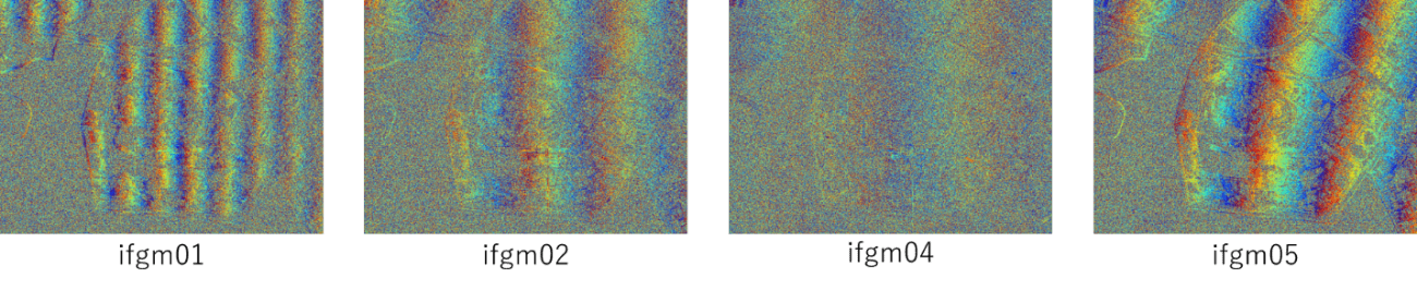
Original data provided by JAXA
Look at the pretty striped pattern this makes. This is a phenomenon called interferometric fringe. Notice how the shapes of the strips on each of the four interferograms differs. We will explain why this happens later on.
This could be considered a sufficient interference, despite being performed at an alignment of one pixel. The part where the strips can’t be distinguished is primarily water surface area, that is, a surface that is considered to have “low coherence”.
We used four different pairs to make our interferograms, but it looks like the fringed pattern in the upper left-hand (ifgm01) and upper right-hand (ifgm05) pictures are relatively easier to read. We will use these data points in the following article. The other two interferograms appear to be less coherent, likely due to insufficient alignment.
These images, however, don’t provide enough information to be useful as data. We still have one more step before we are finished. That is to remove the interferometric fringe.
(4) Removing the Orbital Fringe to Detect Changes within Earth Surface
First, let’s explain what the interferometric fringe is. There are two types of interferometric fringe, with the first being called the “topographic fringe” which gets its name from the bumpy surface caused by hills and mountains. A digital elevation model (DEM) is generally used to create terrain bands in order to delete them from the interferogram. This time, however, we used a method which uses two interferograms to remove this topographic fringe.
The other component that makes up the interferometric fringe is called the “orbital fringe“. This occurs when the satellite’s position changes ever so slightly between observations. With that in mind, all interferograms will be composed of image pairs taken by satellites which have moved, and thus will always create an orbital fringe, as explained in previous articles.
Please always keep in mind that the interferometric fringe refers to both the topographic fringe and the orbital fringe. Removing both kinds of fringes will allow us to see differences in the earth’s surface over a period of time.
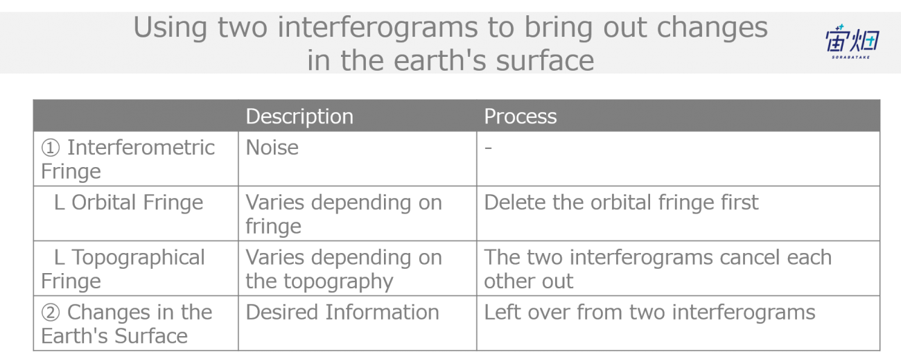
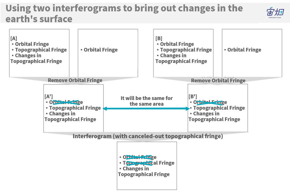
There is a relationship between removing only the topographical fringe, leaving the orbital fringe, and vice-versa. We can detect changes in the earth surface without using external information, such as a DEM, by using this relationship.
To do this, we need two interferograms, and we delete the orbital fringe from one of them, leaving us with the topographic fringe (A’). Then we remove the orbital fringe from the second interferogram, again leaving us only with the topographic fringe (B’). Our process up until now leaves us with A’ and B’, both with a topographic fringe. The topographic fringe is determined by the topography of the image, so A’ and B’ are the same. So if we process the interferogram with A’ and B’, they should cancel each other out. This allows us to process them more easily by only requiring an algorithm for removing the orbital fringe.
Let’s see what kind of changes have been made on the earth’s surface using this method. The best way to remove orbital fringe is to use the information on it. That being said, this method involves a somewhat analog procedure, where we adjust the coefficient for a linear equation of a plane, and then create the orbital fringe in order to remove it.
import numpy as np
import matplotlib.pyplot as plt

def gen_orb(nx,ny,a,b):
    orb = np.zeros([ny,nx])
    for iy in range(ny):
        for ix in range(nx):
            orb[iy,ix] = a*iy+b*ix
    orb = wraptopi(orb)
    return orb

def main():
#インターフェログラムの入力。相感度の強かった01と05を使用する
    ifgm01 = np.load('ifgm01.npy')
    ifgm05 = np.load('ifgm05.npy')

    ny = ifgm05.shape[0]
    nx = ifgm05.shape[1]

    #軌道縞の生成
    orbit01 = gen_orb(nx,ny,-0.00085,-0.044)
    orbit05 = gen_orb(nx,ny,-0.0036,-0.017)

    #軌道縞の削除(3π/4の係数は、画像の中央値を0に近づけるための補正値)
    ifgm01_orb = wraptopi(ifgm01 - orbit01 - np.pi*3/4.)
    ifgm05_orb = wraptopi(ifgm05 - orbit05 + np.pi*3/4.)

    #軌道縞を削除した画像とで差分干渉処理を行い、地形の変化成分を抽出
    difgm = wraptopi(ifgm01_orb - ifgm05_orb - np.pi*3/4.0)

    #画像の保存
    plt.imsave('orbit01.jpg', orbit01, cmap = "jet")
    plt.imsave('orbit05.jpg', orbit05, cmap = "jet")
    plt.imsave('ifgm01_orb.jpg', ifgm01_orb, cmap = "jet")
    plt.imsave('ifgm05_orb.jpg', ifgm05_orb, cmap = "jet")
    plt.imsave('difgm.jpg', difgm, cmap = "jet")


if __name__=="__main__":
       main()
The image produced by running this program can be seen below.
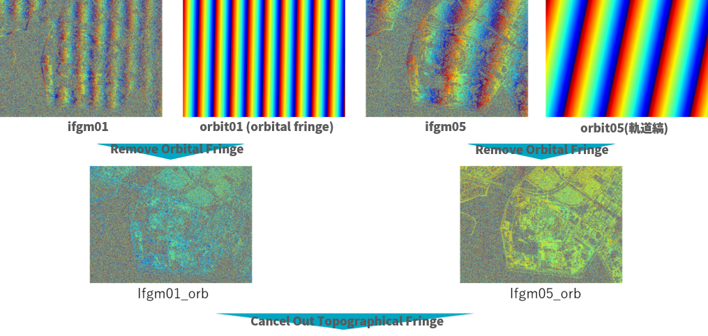
Original data provided by JAXA
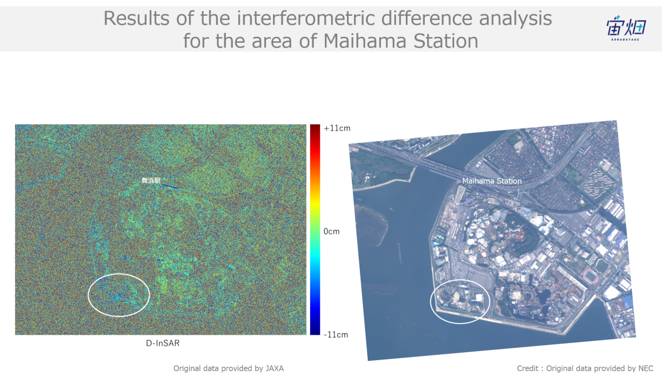
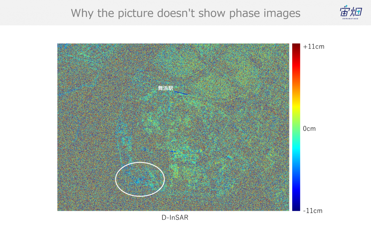
The correlation coefficient has decreased by the final part of our interferometric process, making it harder to see, but looking around the Maihama Station area (green = 0 cm), the area with the white border is showing up slightly blue, which indicates a subsidence of the earth’s surface of a few centimeters. To play into this, product No. 1 was taken on 3/22/18, with product No. 5 was taken on 3/22/19, which sets them about a year apart.
Although there is a large difference in time taken, a report made by the Geospatial Information Authority of Japan shows that this area has seen land subsidence of a few centimeters, which supports the accuracy of our test’s results.
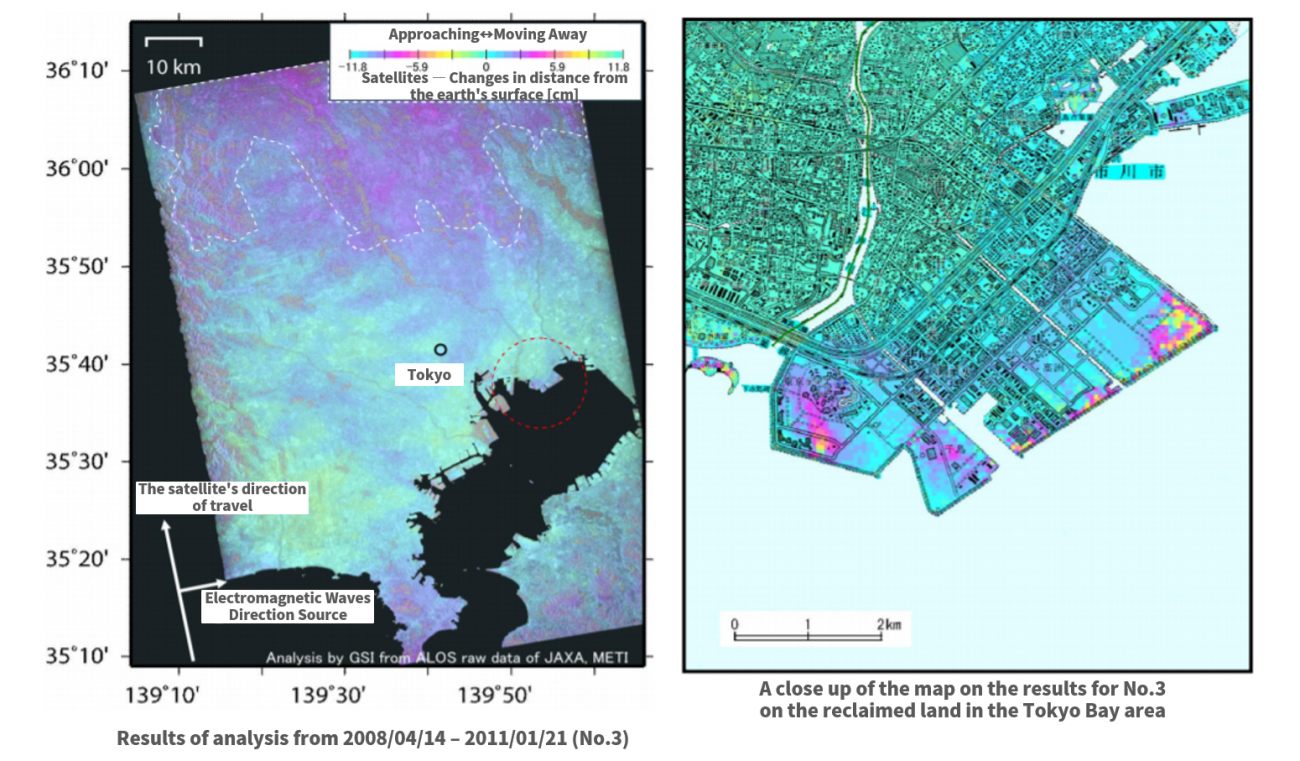
https://vldb.gsi.go.jp/sokuchi/sar/result/sar_data/report/H23_kanshi.pdf
Summary
Let’s finish off this article with a recap on the flow of processing InSAR images. The simple algorithm introduced in this article isn’t as advanced as ones used for research or business. That being said, by following this process, it is possible for users to upgrade this algorithm into their own, original InSAR application.
We hope that our readers try their hand at processing InSAR data on Tellus, and that it will be useful in their businesses and research.
Try using satellite data on "Tellus"!
Want to try using satellite data? Try out Japan’s open and free to use data platform, “Tellus”!
You can register for Tellus here