Tellus has released a function to distribute original data from the satellite data provider in addition to the tiled data that can be easily checked with Tellus OS (on the browser).
For further information, please read this article.

Original data is a difficult thing to handle without knowledge of satellite data, but if you know how to use it, the range of what you can do will expand dramatically.
This article will explain how PALSAR-2 L2.1 processing data available on Tellus is gathered, and how the land coverage is calculated using multifaceted polarized data. The second half will evaluate the results of machine learning.

What is PALSAR-2's Process Level L2.1?

L2.1is an enhanced image that has been processed with resolution and ortho-correction

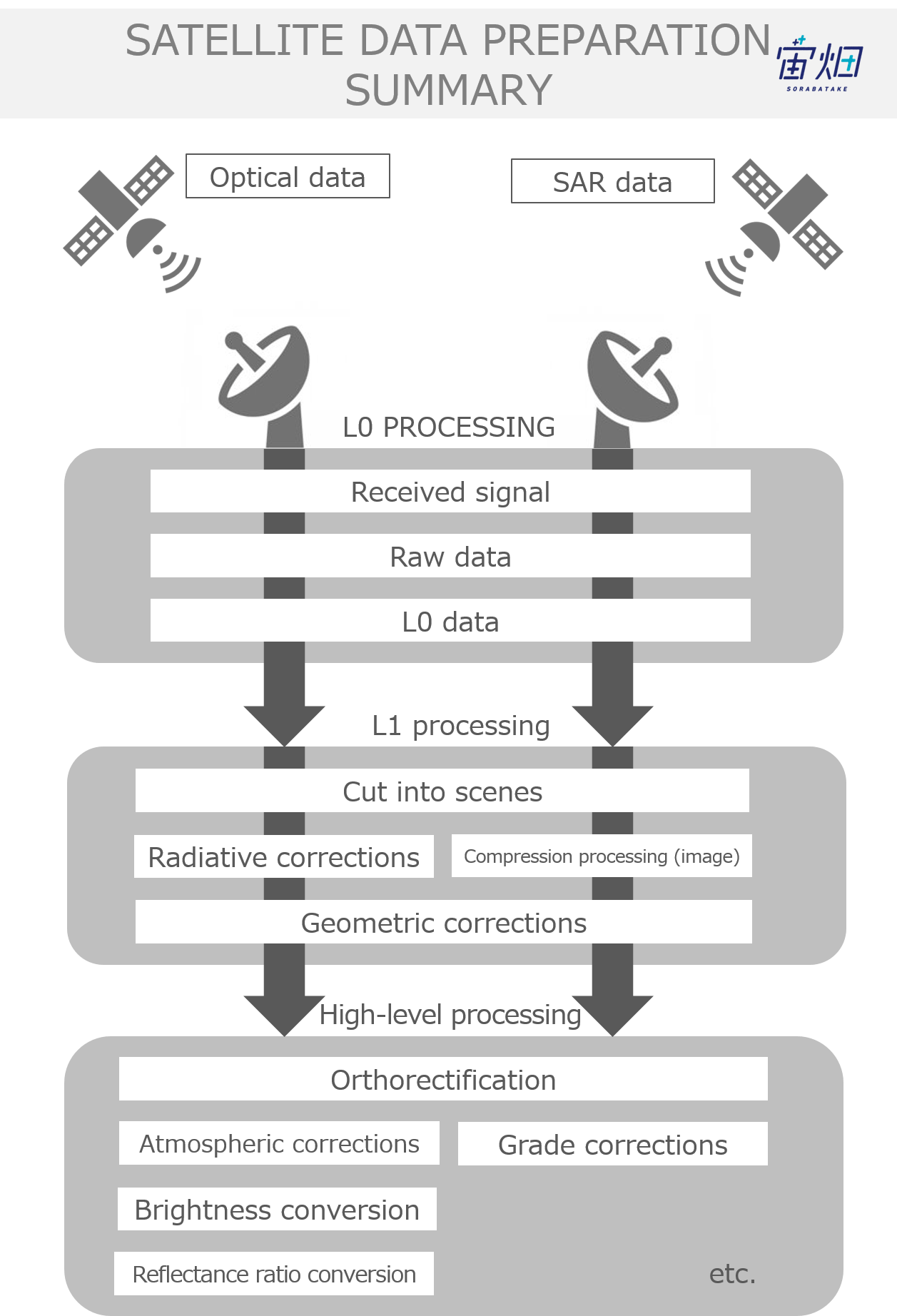
There are several processing levels for SAR images. L2.1 is the high level base product received after performing resolution and ortho-correction to an image. While the information is limited to enhanced information received by electromagnetic waves, the image produced is similar to an optic image, meaning this processing level is capable of being used for various applications such as land coverage detection, vegetation classification, and object detection.

The Key is in the Polarized Data

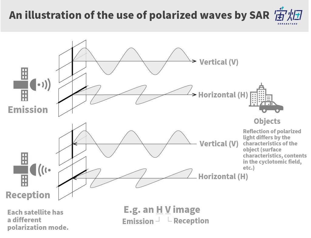
There are a maximum of 4 types of data determined by the type of electro-magnetic wave correspondence called polarized waves (HH, HV, VH, VV). They indicate whether it is a vertical polarization (V) or a horizontal polarization (H) with respect to transmission (1st letter) and reception (2nd letter) respectively. This not only enhances the reception, but makes it possible to analyze images according to their polarization traits.

For more information about SAR data pre-processing, check on the article below.

Let's Gather PALSAR-2 L2.1 Processing Data

See Tellusの開発環境でAPI引っ張ってみた (Use Tellus API from the development environment) for how to use the development environment (JupyterLab) on Tellus.

Downloading the Data Set and Getting a Product ID

In order to download PALSAR-2’s L2.1 products, you need to enter the product ID. All you need to do is look up the product you like and enter its product ID. We will try looking up a product that has multifaceted polarized data recorded on it.

import requests
 
TOKEN = "自分のAPIトークンを入れてください"
 
def search_palsar2_l21(params={}, next_url=''):
    if len(next_url) > 0:
        url = next_url
    else:
        url = 'https://file.tellusxdp.com/api/v1/origin/search/palsar2-l21'
    headers = {
        "Authorization": "Bearer " + TOKEN
    }
	
    r = requests.get(url,params=params, headers=headers)
    if not r.status_code == requests.codes.ok:
        r.raise_for_status()
    return r.json()
 
def main():
    for k in range(100):
        if k == 0:
            ret = search_palsar2_l21({'after':'2017-1-01T15:00:00'})
    	else:
            ret = search_palsar2_l21(next_url = ret['next'])    	
        for i in ret['items']:
            if len(i['polarisations']) > 1:
                print(i['dataset_id'],i['polarisations'])
        if 'next' not in ret:
            break
	
if __name__=="__main__":
       main()

Through using this program, products from after 2017 with more than two types of polarized data can be produced. Choose one of those product IDs and download the data set included in the product with the code below.

import os, requests
 
TOKEN = "自分のAPIトークンを入れてください"
 
def publish_palsar2_l21(dataset_id):
    url = 'https://file.tellusxdp.com/api/v1/origin/publish/palsar2-l21/{}'.format(dataset_id)
    headers = {
    "Authorization": "Bearer " + TOKEN
    }
    r = requests.get(url, headers=headers)
    if not r.status_code == requests.codes.ok:
    r.raise_for_status()
    return r.json()
 
def download_file(url, dir, name):
    headers = {
        "Authorization": "Bearer " + TOKEN
    }
    r = requests.get(url, headers=headers, stream=True)
    if not r.status_code == requests.codes.ok:
        r.raise_for_status()
    if os.path.exists(dir) == False:
        os.makedirs(dir)
        with open(os.path.join(dir,name), "wb") as f:
        for chunk in r.iter_content(chunk_size=1024):
            f.write(chunk)
 
def main():
    dataset_id = 'ALOS2236422890-181009' #選んだプロダクトIDを入力
    print(dataset_id)
    published = publish_palsar2_l21(dataset_id)
    for file in published['files']:
        file_name = file['file_name']
        file_url = file['url']
        print(file_name)
        file = download_file(file_url, dataset_id, file_name)
    print('done')
 
if __name__=="__main__":
    main()

That is all you need to do to gather the data. A folder with the same name as the product ID will be made in the Current Directory containing the data inside of it.

Looking at Land Coverage Data with Polarized Data

Let’s make the polarized data easy to see. This time we use data with HH and HV polarizations, so let’s show the true colors of the data using a combination of the two and their differences. By doing this, we can look up if there is a correlation with different kinds of land coverage for each of the polarized traits

from osgeo import gdal, gdalconst, gdal_array
import os
%matplotlib inline
import numpy as np
import matplotlib.pyplot as plt
 
def normalization(arr):
    min = np.amin(arr)
    max = np.amax(arr)
    ret = (arr-min)/(max-min)
    return ret
 
dataset_id = 'ALOS2236422890-181009'
offx = 14000
offy = 16000
cols = 5000
rows = 5000
 
tif = gdal.Open(os.path.join(dataset_id,'IMG-HH-'+dataset_id+'-UBDR2.1GUD.tif'), gdalconst.GA_ReadOnly)
HH = tif.GetRasterBand(1).ReadAsArray(offx, offy, cols, rows)
tif = gdal.Open(os.path.join(dataset_id,'IMG-HV-'+dataset_id+'-UBDR2.1GUD.tif'), gdalconst.GA_ReadOnly)
HV = tif.GetRasterBand(1).ReadAsArray(offx, offy, cols, rows)
HH = 10*np.log(HH) - 83.0
HV = 10*np.log(HV) - 83.0
HH = normalization(HH).reshape(rows*cols,1)
HV = normalization(HV).reshape(rows*cols,1)
HHHV = normalization(HH-HV).reshape(rows*cols,1)
img = np.hstack((HH,HV,HHHV)).reshape(rows,cols,3)
 
plt.figure()
plt.imshow(img, vmin=0, vmax=1)
plt.imsave('sample.jpg', img)

This is what it looks like if you compare the image we get to one taken by AVNIR-2 on Tellus.

We have chosen an image of the area around Suwako Lake as an example. HH is red and HV is green, and you can see that the city area has a stronger HH reading, and the forest area has much more green. Furthermore, Suwa Lake has weaker reflection levels, making it darker. You can see how this can be used to categorize land coverage to an extent even with only two types of polarized waves.

Predicting Land Coverage with Machine Learning

We used machine learning to show how this can be used. Using the results of the categorization of land coverage performed by JAXA, we have made a prediction model for using machine learning to categorize land coverage.

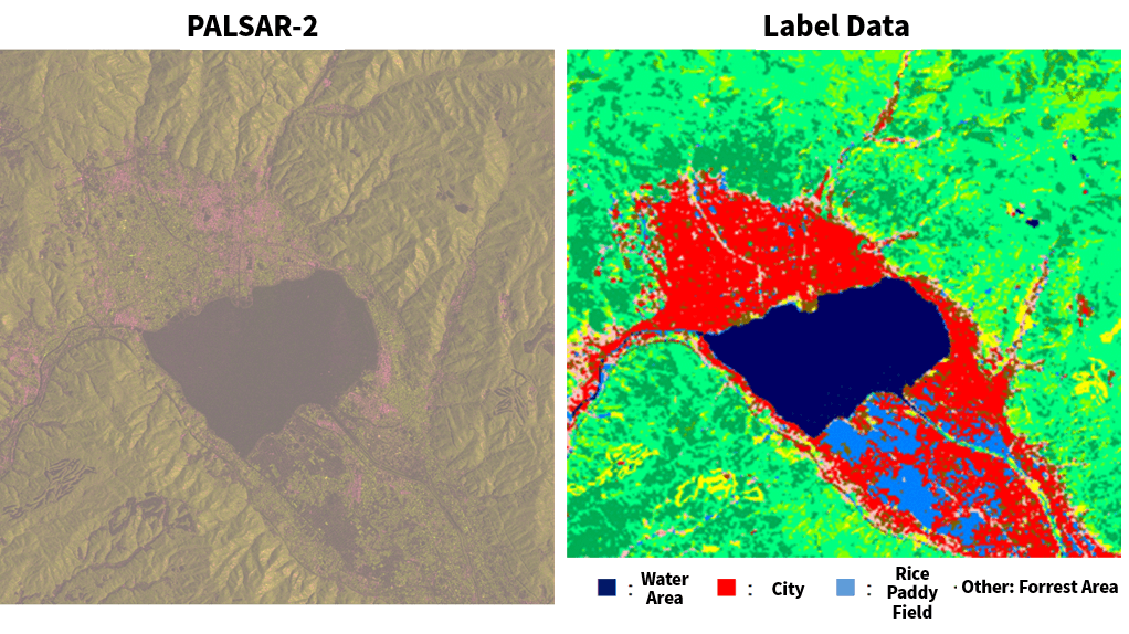
This is what the image that is used for label data looks like.

There are actually ten different classes for this label data, but as the resolution of the label data we are using this time is on the lower end at 30m, and there being only three data points (HH, HV, HH-HV), we graded down to only having the 4 catergories of “water area” “city” “rice paddy field” and “other.”

Data set/How to use CNN

The satellite image and the label image are both formatted as Geotiff, which makes it possible to get the longitude and latitude of each pixel of both of the images. Due to varying resolutions, however, it is necessary to over sample the label data with the lower resolution. The steps to do that are laid out below.

(1) Prepare an empty two-dimensional array with the same number of pixels as the satellite image.
(2) Search for a pixel from a label image that includes the longitude and latitude for each pixel in the satellite image.
(3) Save the label data for that cell into the empty array prepared for (1)

That is how you create label data with the same resolution as satellite images. It doesn’t take long to scan all of the pixels with a for-loop, so anyone can use the steps above to create data.
The learning model includes a CNN constructed with Keras and Tensorflow as referred to in another Sorabatake article. We created a data set of 621 200 x 200 pixel images broken down from a 5400 x 4600 pixel image of Shuwa Lake. This is over sampling the 30m resolution labels to match the resolution of the satellite image. This is split up into practice samples, verification samples, and test samples at a ratio of 7:2:1, respectively.
We took this data and saved it on a Jupyter Notebook to perform machine learning on it. That means we can’t send the files to a third party during the start of the learning phase. Specifically, the array below has been saved as Numpy Array in order to have machine learning performed on it. Inside the () contains the size of the Numpy Array arrangements. We can also easily change the ratio and pixel numbers.

Practice Samples:

X_train（435, 200, 200, 3）

Y_train（435, 200, 200, 4）

Verification Samples:

X_train（124, 200, 200, 3）

Y_train（124, 200, 200, 4）

Test Samples:

X_train（63, 200, 200, 3）

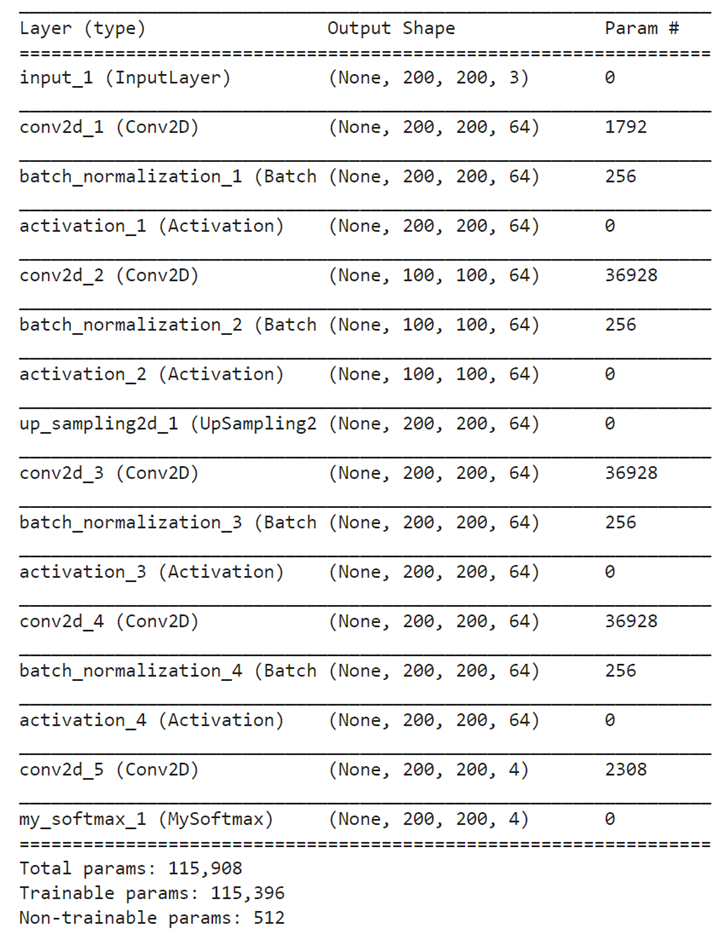
Y_train（63, 200, 200, 4）

The constructed CNN is as follows. After creating the data set, try performing it.

import tensorflow as tf
import keras
from keras import backend as K
from keras.layers import Input, Dropout, Dense, Dropout, Flatten
from keras.layers import Conv2D, MaxPooling2D, UpSampling2D, Activation
from keras.layers.normalization import BatchNormalization
from keras.models import Model
from keras.activations import softmax
from keras.engine.topology import Layer

class MySoftmax(Layer):
    def __init__(self, **kwargs):
        super(MySoftmax, self).__init__(**kwargs)
    def call(self, x):
        return(softmax(x, axis=3))

# parameter
img_size = 200
npol = 3
nclass = 4


# create model
input_shape = (bsize, bsize, npol)
input = Input(shape=input_shape)
act = 'relu'
net = Conv2D(filters=64, kernel_size=(3,3), strides=(1,1), padding="same", kernel_initializer="he_normal")(input)
net = BatchNormalization()(net)
net = Activation(act)(net)
net = Conv2D(filters=64, kernel_size=(3,3), strides=(2,2), padding="same", kernel_initializer="he_normal")(net)
net = BatchNormalization()(net)
net = Activation(act)(net)
net = UpSampling2D((2,2))(net)
net = Conv2D(filters=64, kernel_size=(3,3), strides=(1,1), padding="same", kernel_initializer="he_normal")(net)
net = BatchNormalization()(net)
net = Activation(act)(net)
net = Conv2D(filters=64, kernel_size=(3,3), strides=(1,1), padding="same", kernel_initializer="he_normal")(net)
net = BatchNormalization()(net)
net = Activation(act)(net)
output = Conv2D(filters=nclass, kernel_size=(3,3), strides=(1,1), padding="same", kernel_initializer="he_normal")(net)# class
output = MySoftmax()(output)
model = Model(input, output)

## optimizer
opt= keras.optimizers.Adam(lr=1e-3)
model.compile(loss="sparse_categorical_crossentropy", optimizer=opt)
print(model.summary())

##実際のデータを用いた学習（実行するには、事前にデータの作成が必要です）
model.fit(X_train, Y_train, batch_size=16, epochs=24, validation_data=(X_val, Y_val))

After conducting machine learning, and evaluating the test images, this is what we got.

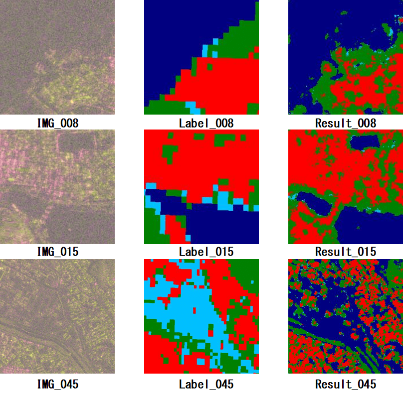
Looking at the results, the shore of the Shuwa Lake has higher definition than the teacher label. Furthermore, the city area with high levels of red (HH polarization), and the forest area with high levels of green (HV polarization) appear to have much finer resolution and accuracy than the label. Unfotunately, almost all of the light blue rice paddy fields came out as the same color as the water area. It looks like using the combination of only HH and HV aren’t strong enough to pick up these differences.
According to research on machine learning that uses SAR data, using HV and VV waves, which have differing phase contrast in their corresponding polarizations is effective. In order to use phase information, you need to use L1.1 information introduced in our last article, which you can read here.

Summary

This article explained how to use SAR data to calculate land coverage and make its data visible. You can see how just like optic images, SAR can also have machine learning conducted on it using multifaceted polarization information.
While it was a simple example, this should give you a picture of how SAR data and AI work together. The practical use for SAR images is considered to be in a developmental stage compared to optics. Definitely try using the standard processing product available for use on Tellus.