For readers who want to try using machine learning and satellite data to do something interesting, we’d like to suggest trying out object detection.

In this article, we have attempted to use satellite data in order to perform object detection on airplanes. Being able to detect airplanes could allow us to do things like make estimates on how many people use airports only using satellite data.  We could potentially use the same method on boats, or cars to figure out how many cars are in a parking lot.

You’ll be able to detect airplanes too if you just follow the code laid out in this article. There are some parts of our process that aren’t entirely optimal, so we would like to welcome any comments and feedback from our readers.

With that said, let’s begin!

1. What is Object Detection?

Let’s start by explaining what exactly object detection is? You may know of “image classification”, which is a technique that takes objects captured in photos and puts them into categories, such as cats and dogs.  Object detection differs from this in that it doesn’t only categorize what is being shown in the photo, but also shows what and where something is.

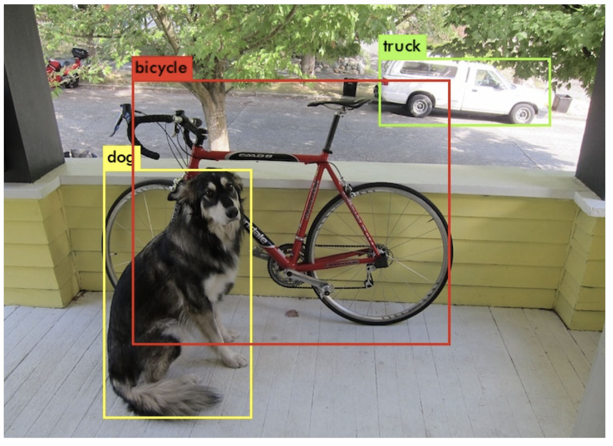
One example where this technology is often used is for detecting boats. In fact, Tellus holds a competition called the “Tellus Satellite Challenge”, where one of the themes in the past was boat detection. You can read our article on that here. Object detection can also be used to detect vehicles or the exact location of landslides in times of disaster, making it an important technology in a wide variety of fields.

2. How to Perform Object Detection

There are lots of ways to perform object detection. Here is the most well-known method. Most other methods are subsets of this.

- R-CNN (R-CNN, Fast R-CNN, Faster R-CNN)):

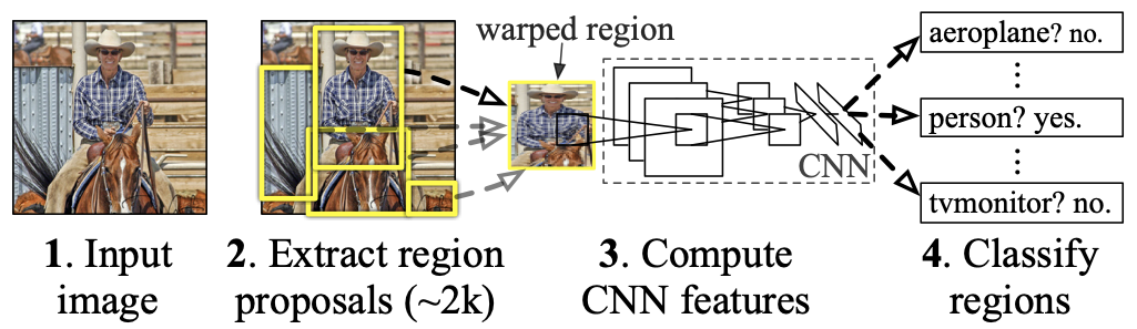
R-CNN (you can read the full thesis here) was a pioneer method for bringing CNN to object detection. First it performs what’s called a selective search to break down the image into segments that likely contain objects, then CNN is used to extract their features. After that, SVM (support vector machine) is used to classify the objects by the extracted features.

“Fast R-CNN” and “Faster R-CNN” have been designed to speed up calculations by using CNN to narrow down the segments and classify objects.

YOLO (you can read the full thesis here):

YOLO, on the other hand, is different from R-CNN  in that it uses a single network to break the image into segments and classify objects, as opposed to R-CNN which breaks this process into two steps. In other words, the single network is capable of both creating the coordinates for the bounding box and determining the classification for the object it holds at the same time. This shortens the amount of time it takes to calculate the images, making the whole process go by much quicker.

– SDD (you can read the full thesis here):

This is the same as YOLO in that it uses a single network to detect segments and classify them. By making feature maps of various sizes, it’s possible to get predictions for a different variety of sizes for the objects shown within the image. This is the method we will be using in this article.

To learn more about these different methods, you can check out Tellus Trainer, which has explanations using videos and available code.

3. The Flow for Implementing SSD Code and General Overlay

We’ll explain how to implement the code using the following steps.

Step 1: Download the learning data
Step 2: Prepare the data
Step 3: Create a Dataset
Step 4: Create the DataLoader
Step 5: Create a SSD Model
Step 6: Define the loss function, and set the optimization method
Step 7: Run the learning/verification process
Step 8: Compare it with the test data

We used the machine learning library, PyTorch, for implementation. The code we used in the article is available on GitHub, and by running the following command you can copy the code into your own development environment.

git clone https://github.com/ryomaouchi/SSD_airplane_sorabtake

To create the code, we used the book “Learn as you go! Deep Learning with Pytorch” as a reference while we tackled the task at hand. The code itself is based on the code in the book’s support repository, but please be aware that there are many parts that we have altered.

Below is a general overlay of the code. (The dataset_rareplanes and weights directories aren’t on GitHub and will be made within the main.ipynb). Supplementary descriptions have been written in blue for each directory and file.

┣ main.ipynb
┃ (#code that describes the main flow. It will generally follow this flow)
┃
┣ Dataset_rareplanes (a directory of the synthetic teaching data for #RarePlanes)
┃　      ┣ train (#insert learning data)
┃        ┃  ┣ images
┃        ┃  ┗ labels
┃        ┣ val (#insert verfication data) 
┃        ┃  ┣ images
┃        ┃  ┗ labels
┃        ┗ test (#insert valuation data)
┃              ┣ images
┃              ┗ labels
┃
┣ utils  (#store the group of files that contain the various classifications and functions)
┃  ┣ augumentation.py (#supplement the data)
┃  ┣ dataloader.py (#set the definitions for the dataset and dataloader)
┃  ┣ ssd_model.py (#write the contents of the SSD model)    
┃  ┣ loss.py (#define the loss function)
┃  ┗ ssd_predict_show.py (#show the predictions made by the learned model)
┃
┗ weights (#save model gained through learning here)

4. Implementing the Code

The overall flow for the code is enscribed in the main.ipynb file, and if you implement this code you’ll be able to perform object detection. When you do this, the classes and functions you’ll need are saved in a group of files which can be found in the utils directory, you can use these where you need to when using the main.ipynb.

This article will go over primarily main.ipynb. The details about the classes within the utils directory can be found in the supplementary explanations on the comments in the code and our reference book.

We’ll be conducting our calculation on the following Tellus environment.

#########################################

– Exclusive environment (Sakura’s dedicated server)
– CPU: Xeon Silver 4114 10core 2.20 GHz
– memory: 96GB
– disk (raid1): SSD480GB + SSD960GB

#########################################

We also confirmed that the code works on Tellus’s test environment plan which has 8 GB of memory, so you should be able to use it on whatever environment you are using.

Let’s check out all of the contents of main.ipynb in order.

[Installing the required libraries]

Let’s start by installing the required libraries.

!pip install torch==1.0.1
!pip install torchvision==0.2.1

import numpy as np
import matplotlib.pyplot as plt
%matplotlib inline
import os
import sys
import time 
import pandas as pd
import urllib.request
import zipfile
import tarfile
import cv2
import random
import xml.etree.ElementTree as ET
from math import sqrt
from glob import glob
from itertools import product


import torch
import torch.utils.data as data
import torchvision
import torch.nn as nn
import torch.nn.functional as F
import torch.nn.init as init
import torch.optim as optim
from torch.autograd import Function

# utilsというディレクトリ中のファイルから必要なコードをインポートする。
from utils.augmentations import Compose, ConvertFromInts, ToAbsoluteCoords, PhotometricDistort, Expand, RandomSampleCrop, RandomMirror, ToPercentCoords, Resize, SubtractMeans
from utils.dataloader import RareplanesDataset, DataTransform, xml_to_list, od_collate_fn, get_color_mean

[Step 1: Downloading the teaching data]

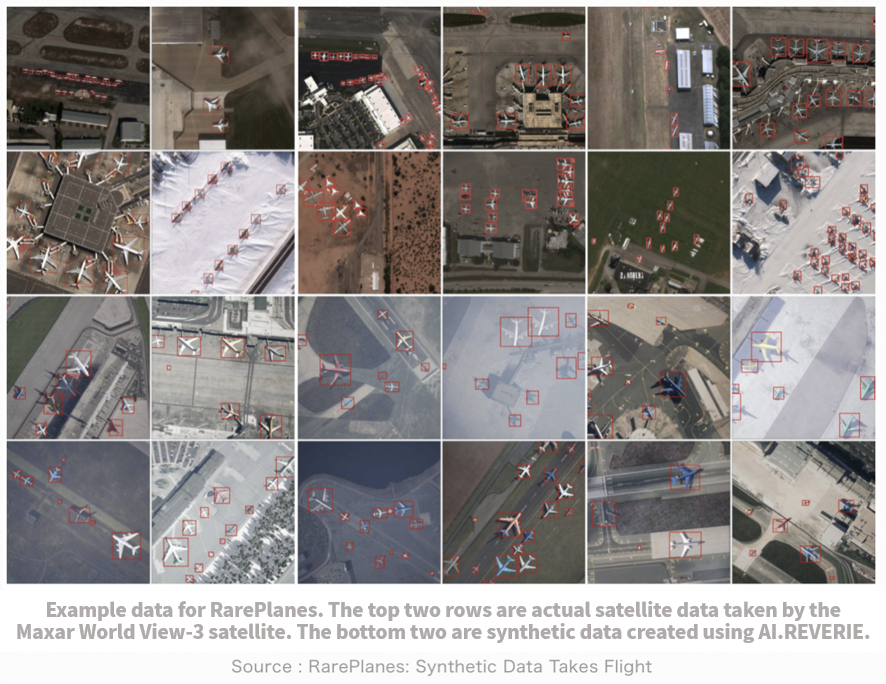
Next, we will download the teaching data that we will use to learn. This time we’ll be using a public data set called RarePlanes used for detecting airplanes. You can find out more about RarePlanes in a previous Sorabatake Article in which we go into detail about the data set.

RarePlanes includes large amounts of synthetic teaching data in addition to Real-World satellite data from Maxar Worldview-3. Synthetic teaching data is an artificially created image used for teaching used to supplement or replace the actual satellite data used for learning. We’ll be using the synthetic RarePlanes data for our learning.

As is written in the general layout for our code, first we create a Data_rareplanes

directory for putting data into, and then within that directory, we create three more directories: train, val, and test.

Downloading all of the synthetic Rareplane data takes up more than 211 GB, so we’ll just download a portion of it. Pick out all of the images that end in 10, 20, or 30 and download them from the AWS. The size of the data is 5.3 GB.

The development environment provided on Tellus doesn’t allow us to bring the data directly due to authentication reasons, so this time you’ll have to upload the data locally before uploading it to the Tellus development environment. You can download the data locally by hitting the following command on your PC.

#学習用データのダウンロード
aws s3 cp --recursive s3://rareplanes-public/synthetic/train/images ./Data_rareplanes/train/images/ --exclude "*.png" --include "*10.png" 
aws s3 cp --recursive s3://rareplanes-public/synthetic/train/xmls ./Data_rareplanes/train/labels/ --exclude "*.xml" --include "*10.xml"

#検証用データのダウンロード
aws s3 cp --recursive s3://rareplanes-public/synthetic/train/images ./Data_rareplanes/val/images/ --exclude "*.png" --include "*20.png" 
aws s3 cp --recursive s3://rareplanes-public/synthetic/train/xmls ./Data_rareplanes/val/labels/ --exclude "*.xml" --include "*20.xml"

#評価用データのダウンロード
aws s3 cp --recursive s3://rareplanes-public/synthetic/train/images ./Data_rareplanes/test/images/ --exclude "*.png" --include "*30.png" 
aws s3 cp --recursive s3://rareplanes-public/synthetic/train/xmls ./Data_rareplanes/test/labels/ --exclude "*.xml" --include "*30.xml"

Note that running this code requires an AWS account and certain configurations. For details, check the main.ipynb.

With this, the teaching data is now ready.

[Step 2. Preparing the Images]

Let’s talk about what we mean by preparing the data.

To prepare the images, you’ll have to implement a call called DataTransform. This class is written in the dataloaders.py, so you can check the details there. We’ll cover just the main points in this article.

In the SSD model that we’ll implement today, we’re assuming the size of the input image is 300×300. So for this class, we’ll have to resize the images to match our dimensions.

We’ll also have to subtract the average color data for each channel (B, G, R) in order to standardize the data. In order to do that, you’ll need the average pixel values for each channel for every learning image. The function used to calculate that is the get_color_mean, which can be found in dataloader.py.

Finally, you’ll generally want to enhance your learning data, which is known to improve the accuracy of learning models. You can enhance it by using DataTransform. What happens when you do this is it takes random parts of random images, changes their colors, and inverts them to be used as learning images.

[Step 3. Creating the Data Set]

Next, we will create the data set. This is done in a class called RareplanesDataset (a detailed implementation can be seen in dataloaders.py).

We’ll start off by taking the learning image and its annotation (which is a teaching label) file, as well as the verification image and its annotation file and storing their paths in each list.

train_image_dir = './Data_rareplanes/train/images/'
train_img_paths = glob(os.path.join(train_image_dir, '*.png'))
#学習用画像ファイルのパスリスト

val_image_dir = './Data_rareplanes/val/images/'
val_img_paths = glob(os.path.join(val_image_dir, '*.png'))
#検証用画像ファイルのパスリスト


train_label_paths = [train_img_paths[i].replace('png', 'xml',1).replace('images','labels',1) for i in range(len(train_img_paths))]
#学習用データのアノテーションファイルのパスリスト

val_label_paths = [val_img_paths[i].replace('png', 'xml',1).replace('images','labels',1) for i in range(len(val_img_paths))]
#検証用データのアノテーションファイルのパスリスト

Then we will take the classes we will be working with and make a list (although we are only working with on class this time, lol).

my_classes = ["airplane"]

The airplane annotation data for each image is written in an .xml file. You’ll know when you look at the file, but it contains lots of different data.

From this file, we’ll take the class for extracting the list of the bounding box data for each airplane, and save it as “xml_to_list” to the dataloaders.py. Bounding boxes are the four corners of the squares that will surround the planes.

Now we will be using these functions and classes to define the following data set.

input_size = 300 #今回は入力画像を300×300にする

#学習用データセットの定義
train_dataset = RareplanesDataset(train_img_paths, train_label_paths, phase = 'train', transform = DataTransform(input_size, color_mean), transform_anno = xml_to_list(my_classes))

#検証用データセットの定義                               
val_dataset = RareplanesDataset(val_img_paths, val_label_paths, phase = 'val', transform = DataTransform(input_size, color_mean), transform_anno = xml_to_list(my_classes))

[Step 4. Creating the Data Loader]

Next we will take data from the data sets we defined above and create data batches (small groups of data) in order to define the data loader. Our batch size for this is 32.

batch_size = 32 

train_dataloader = data.DataLoader(
    train_dataset, batch_size = batch_size, shuffle = True, collate_fn = od_collate_fn
)

val_dataloader = data.DataLoader(
    val_dataset, batch_size = batch_size, shuffle = True, collate_fn = od_collate_fn
)

# 辞書型としてまとめておく
dataloaders_dict = {"train": train_dataloader, "val": val_dataloader}

[Step 5. Creating the SSD Model]

Now it’s time for us to define the most important part of the code, the SSD model.

The composition of the SSD network is as follows.

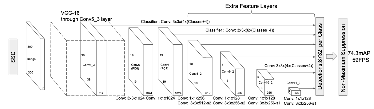
There are too many details for us to dive into in order to describe the implementation of this network, so please see reference 1 and the original thesis for more details. The structure of the network above is configured using Pytorch, and the model can be found in a file called the ssd_model.py in the utils directory.

The network above consists of various layers including a convolution and max pooling layer, but we can use Pytorch to write these layers in with just one line of code. So even complicated networks can be put together like Lego.

Now we’ll take our newly acquired SSD model and set the parameters of the network as follows.

# utils下のssd_model.pyというファイルからSSDというクラスをインポート。
from utils.ssd_model import SSD

ssd_cfg = {
    'num_classes': 2, # 背景も含めるためクラスの数は2。
    'input_size': 300, # 入力画像のサイズは300×300にリサイズしている。
     # 以下のパラメータの詳細は参考文献などをご覧ください。　
    'bbox_aspect_num': [4,6,6,6,4,4], 
    'feature_maps': [38,19,10,5,3,1],
    'steps': [8,16,32,64,100,300],
    'min_sizes': [30,60,111,162,213,264],
    'max_sizes': [60,111,162,213,264,315],
    'aspect_ratios': [[2],[2,3],[2,3],[2,3],[2],[2]]
}

net = SSD(phase='train', cfg = ssd_cfg)

Then we will reset the weights of the networks.

The SSD network partially includes a module based on VGG-16. For this module, you’ll use the weights we learning by sorting Image net images. You can get this trained model from the following URL.

# ディレクトリ「weights」が存在しない場合は作成する
weights_dir = "./weights/"
if not os.path.exists(weights_dir):
    os.mkdir(weights_dir)

# 学習済みモデルをダウンロード
# MIT License
# Copyright (c) 2017 Max deGroot, Ellis Brown
# https://github.com/amdegroot/ssd.pytorch

url = "https://s3.amazonaws.com/amdegroot-models/vgg16_reducedfc.pth"
target_path = os.path.join(./weight, "vgg16_reducedfc.pth") 

if not os.path.exists(target_path):
    urllib.request.urlretrieve(url, target_path)

Once you have the learned model, reset the weights for the network. For modules other than the VGG module, use the initial value of He (reference article here).

# 学習済みモデルで重みを初期化
vgg_weights = torch.load('./weights/vgg16_reducedfc.pth')
net.vgg.load_state_dict(vgg_weights)

def weights_init(m):
    if isinstance(m, nn.Conv2d):
        init.kaiming_normal_(m.weight.data)
        if m.bias is not None:
            nn.init.constant_(m.bias,0.0)
         
# 他の重みはHeの初期値で初期化する   
net.extras.apply(weights_init)
net.loc.apply(weights_init)
net.conf.apply(weights_init)

#使用しているデバイスの定義
device = torch.device("cuda:0" if torch.cuda.is_available() else "cpu")

[Step 6. Define the Loss Function, and Set the Optimization Method]

In order to teach the model, we’ll need to define a loss function to act as an indicator to see how much the values created by the network deviates from the teaching label.

Loss is caused by a combination of predictions for classification and the position of the bounding boxes. For classification predictions, we use a cross-entropy error function, and for bounding box predictions we use an L1 loss function. The implementation is done in a class called MultiBoxLoss, and is described in the loss.py in the utils directory.

# utilsというディレクトリ下のloss.pyというファイルからMultiBoxLossというクラスをインポート。
from utils.loss import MultiBoxLoss

criterion = MultiBoxLoss(jaccard_thresh=0.5, neg_pos = 3, device=device)

We’ll use the Adam function of Pytorch for optimization.

optimizer = optim.Adam(net.parameters(), lr=0.001, betas=(0.9, 0.999), eps=1e-08, weight_decay=0, amsgrad=False)

[Step 7. Learning/verifying the Data]

It’s almost time for us to start the learning. Before we do so, we need to implement the learning details from the train_model function defined below.

def train_model(net,dataloaders_dict, criterion, optimizer, num_epochs):
    # 使用デバイスの定義
    device = torch.device("cuda:0" if torch.cuda.is_available() else "cpu")
    print("使用Device:", device)
    
    # (もしGPUを使用しているなら)ネットワークをGPUに渡す
    net.to(device)
        
    # ネットワークがある程度固定であれば、高速化させる
    torch.backends.cudnn.benchmark = True
    
    iteration = 1
    epoch_train_loss = 0.0
    epoch_val_loss = 0.0
    logs = []
    
    #学習開始
    for epoch in range(num_epochs+1):
        t_epoch_start = time.time()
        t_iter_start = time.time()
    
        print('------------')
        print('Epoch {}/{}'.format(epoch+1, num_epochs))
        print('------------')
     
        for phase in ['train', 'val']:
            if phase == 'train':
                net.train()
                print(' (train) ')
        
            else:
                #10エポックごとに検証用画像に対する損失を表示。
                if ((epoch+1) % 10 == 0):
                    net.eval()
                    print('----------')
                    print(' (val) ')
                    
                else:
                    continue
                    
            for images, targets in dataloaders_dict[phase]:
                images = images.to(device)
                targets = [ann.to(device)
                            for ann in targets]
                    
                optimizer.zero_grad()
                    
                with torch.set_grad_enabled(phase=='train'):
                    outputs = net(images)
                    
                    #損失関数は、バウンディングボックスの位置の予測に関するもの(=loss_l)と分類予測に関するもの(=loss_c)の和になる。
                    loss_l, loss_c = criterion(outputs, targets)
                    loss = loss_l + loss_c
                    
                    if phase == 'train':
                        loss.backward()
                            
                        nn.utils.clip_grad_value_(
                            net.parameters(), clip_value = 2.0
                            )
                            
                        optimizer.step()
                         
                         # 2イテレーションごとにかかった時間と損失を表示。
                        if (iteration % 2 ==0):
                            t_iter_finish = time.time()
                            duration = t_iter_finish - t_iter_start
                            print('イテレーション {} || Loss: {:.4f} || 10iter:{:.4f} sec.'.format(
                            iteration, loss.item(), duration))
                            t_iter_start = time.time()
                            
                        epoch_train_loss += loss.item()
                        iteration += 1
                        
                    else:
                        epoch_val_loss += loss.item()
                                
                                
        t_epoch_finish = time.time()
        print('------------')
        print('epoch {} || Epoch_TRAIN_Loss:{:.4f} || Epoch_VAL_Loss:{:.4f}'.format(
        epoch+1, epoch_train_loss, epoch_val_loss))
        
        print('timer: {:.4f} sec.'.format(t_epoch_finish - t_epoch_start))
        t_epoch_start = time.time()
        
        log_epoch = {'epoch': epoch+1, 'train_loss': epoch_train_loss, 'val_loss': epoch_val_loss}
        logs.append(log_epoch)
        df = pd.DataFrame(logs)
        df.to_csv("log_output.csv")
        
        epoch_train_loss = 0.0
        epoch_val_loss = 0.0
        
        #10エポックごとに重みを保存する。
        if ((epoch+1)%10 ==0):
torch.save(net.state_dict(),'weights/SSD300_'+str(epoch+1)+'.pth')

Let’s start learning using the train_model function defined above.

This time, 200 epochs were used to perform this calculation. The calculation doesn’t need to be this complicated to give you sufficiently accurate results, so for those of you who are feeling impatient, it should be okay to decrease the number of num_epochs (around 50 should be fine).

# 計算するエポック数
num_epochs = 200  

train_model(net, dataloaders_dict, criterion, optimizer, num_epochs = num_epochs)

You should get the following.

使用Device: cpu
------------
Epoch 1/200
------------
 (train) 
イテレーション 2 || Loss: 3509.4802 || 10iter:52.2317 sec.
イテレーション 4 || Loss: 99.7308 || 10iter:53.4657 sec.
イテレーション 6 || Loss: 17.1309 || 10iter:51.2001 sec.
イテレーション 8 || Loss: 30.4145 || 10iter:52.1168 sec.
イテレーション 10 || Loss: 15.8940 || 10iter:52.4673 sec.
イテレーション 12 || Loss: 10.5187 || 10iter:52.4800 sec.
イテレーション 14 || Loss: 9.1825 || 10iter:46.5551 sec.
------------
epoch 1 || Epoch_TRAIN_Loss:3818.9820 || Epoch_VAL_Loss:0.0000
timer: 360.5179 sec.
------------
Epoch 2/200
------------
 (train) 
イテレーション 16 || Loss: 8.4894 || 10iter:50.7820 sec.

. . . . . . . . .

------------
Epoch 201/200
------------
 (train) 
イテレーション 2802 || Loss: 3.1097 || 10iter:54.2413 sec.
イテレーション 2804 || Loss: 3.5624 || 10iter:55.0426 sec.
イテレーション 2806 || Loss: 2.7226 || 10iter:51.6822 sec.
イテレーション 2808 || Loss: 3.2201 || 10iter:51.3310 sec.
イテレーション 2810 || Loss: 2.7209 || 10iter:52.9426 sec.
イテレーション 2812 || Loss: 3.0924 || 10iter:52.6623 sec.
イテレーション 2814 || Loss: 2.9761 || 10iter:46.9799 sec.
------------
epoch 201 || Epoch_TRAIN_Loss:41.8153 || Epoch_VAL_Loss:0.0000
timer: 364.8839 sec.

Be aware that the calculation will end with num_epoch+1.

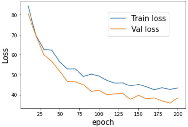
Let’s plot out the changes in the loss function accompanied by the epochs. You can view it with the code below.

#損失関数のプロット

log_data = pd.read_csv("log_output.csv")
#エポック10ごとに切り出す
log_data_10 = log_data[log_data["epoch"] % 10 == 0]

plt.xlabel("epoch", fontsize= 15)
plt.ylabel("Loss", fontsize= 15)

plt.plot(log_data_10["epoch"],log_data_10["train_loss"], label="Train loss")
plt.plot(log_data_10["epoch"],log_data_10["val_loss"], label="Val loss")

plt.legend(bbox_to_anchor=(0.9, 0.9), loc='upper right', borderaxespad=0, fontsize=15)
plt.show()

The result is as shown below. You can see that the loss has decreased for both the learning and verification images, and the curve flattens out the more epochs there are. Also notice that there isn’t a big difference in loss function between the learned images and verification images, meaning that it’s safe to say we didn’t overlearn the data.

[Step 8. Comparing with the test data]

We’ll use the model we learned at the end to detect airplanes in the test images. We’re not going to use an evaluation indicator (like mAP) against the test data in this article, so we’ll pick out two test images to perform inference on. The two photos are a test image of Data_rareplanes and an image of Narita International Airport taken by ASNARO-1.

First, we’ll need to change the settings of our SSD network to inference mode. Then,
we’ll load the final weights we learned above (‘./weights/SSD300_200.pth’). What you have to be careful of here is, if you changed the number of epochs with num_epochs earlier, you’ll also need to change the filename to “SSD300_numberofepochs”.

# ネットワークを推論ように切り替える
net = SSD(phase='inference', cfg = ssd_cfg)

# 上で学習した重みを読み込む
net_weights = torch.load('./weights/SSD300_200.pth', map_location={'cuda:0': 'cpu'})
net.load_state_dict(net_weights)

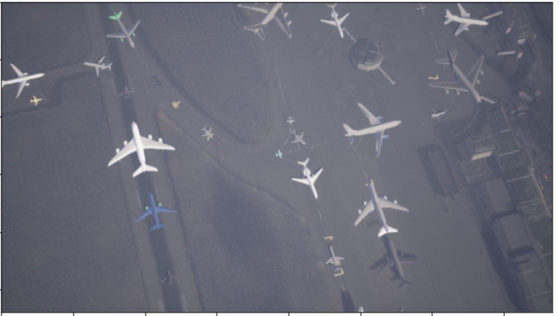
- Picture from Data_rareplanes in the Test Directory

Let’s display the resulting image next to one of our test images.

# 推論結果を表示するためのクラスSSDPredictShowをutils下のssd_predict_show.pyから読み込む
from utils.ssd_predict_show import SSDPredictShow 

test_image_dir = './Data_rareplanes/test/images/'
test_img_paths = glob(os.path.join(test_image_dir, '*.png'))

# 評価用画像を一枚読み込む
img_file_path = test_img_paths[1]
ssd = SSDPredictShow(color_mean, eval_categories = my_classes, net = net)
ssd.show(img_file_path, data_confidence_level=0.3)

Compare the result with the original image.

- Original Image

- Forcasted Results

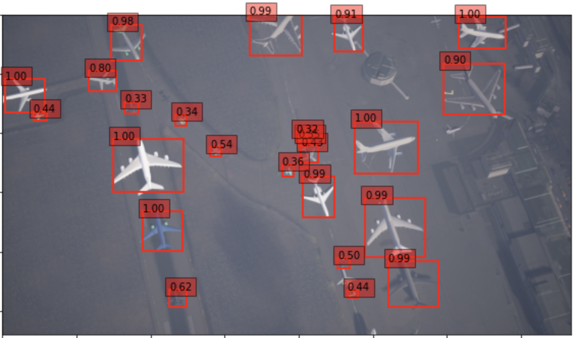
The results look pretty good, you can seen that it even picked up smaller airplanes.

But you’re probably thinking to yourself,
“does using synthetic teaching data to test against synthetic teaching data without an actual image actually give you any real results?”

So for our next image, we’ll test it against a picture taken by the ASNARO-1 satellite.

- Image of Narita International Airport taken by ASNARO-1

First, we’ll have to download an ASNARO-1 image from the Tellus development environment. Use the following code on the development environment to save a picture of Narita International Airport.

For this image, we set the zoom to 17, and combined 3 x 3 tiles to create our image. You can learn how to combine tiles to create images in this Sorabatake article.

import requests
from skimage import io
from io import BytesIO
%matplotlib inline
TOKEN = "(自分のトークンを貼り付ける)"

def get_combined_image(get_image_func, z, topleft_x, topleft_y, size_x=1, size_y=1, option={}, params={}):
    rows = []
    blank = np.zeros((256, 256, 4), dtype=np.uint8)
    
    for y in range(size_y):
        row = []
        for x in range(size_x):
            try:
                img = get_image_func(z, topleft_x + x, topleft_y + y, option, params)
            except Exception as e:
                img = blank
                
            row.append(img)
        rows.append(np.hstack(row))
    return  np.vstack(rows)

def get_asnaro1_image(z, x, y, option, params={}):
    url = 'https://gisapi.tellusxdp.com/ASNARO-1/{}/{}/{}/{}.png'.format(option['entityId'], z, x, y)
    headers = {
        'Authorization': 'Bearer ' + TOKEN
    }
    r = requests.get(url, headers=headers, params=params)
    if not r.status_code == requests.codes.ok:
        r.raise_for_status()
    return io.imread(BytesIO(r.content))    

option = {
    'entityId': '20190110093424839_AS1' # 成田国際空港が写っているシーン
}
z = 17       # ズーム率
x = 116650    # 起点となるタイルのx座標
y  = 51570  # 起点となるタイルのy座標

#起点となるタイルから3×3枚のタイルを結合
combined = get_combined_image(get_asnaro1_image, z, x, y, 3, 3, option)

#io.imshow(combined)
io.imsave('./Narita_airport_ASNARO1_zoom17.png', combined)

Running the code will have you download a file　called “Narita_airport_ASNARO1_zoom17.png”.

Let’s run our learned model against the ASNARO-1 image you acquired above.

from utils.ssd_predict_show import SSDPredictShow 

img_file_path = "./Narita_airport_ASNARO1_zoom17.png"
ssd = SSDPredictShow(color_mean, eval_categories = my_classes, net = net)
ssd.show(img_file_path, data_confidence_level=0.3)

Here is a comparison of the results (left: original image, right: our prediction).

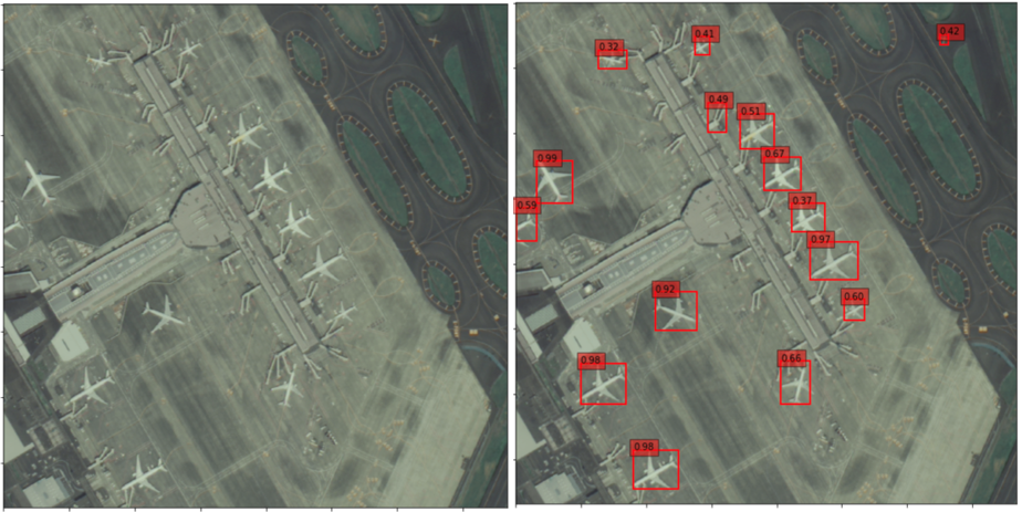
There are a few mis-detections, but you can see that it was able to detect all of the airplanes. It is pretty interesting how we were able to get such accurate results when we didn’t even use satellite data for our machine learning.

5. Discussion and Future Considerations

In this article, we used a synthetic teaching data set called RarePlanes to create an SSD learning model for detecting airplanes. When running our learning model against actual satellite images taken by ASNARO-1, we were able to detect airplanes with considerable accuracy.

We could potentially use this learning model to count the number of planes currently in airports to calculate the impact of the coronavirus on the number of flights. For more information on solving such tasks, you can find out more information on this page about using Sentinel-1 satellite images.

In this article, we detected airplanes, but it might be interesting to try detecting other objects as well.

For example, you could look into the number of cars parked at a shopping mall. By monitering the daily changes in parking lot traffic, you could potentially calculate the profits made by that shopping mall. This could also be used for golf courses, wine fields, oil tankers, and a variety of other fields to produce potentially interesting results.

There are lots of ways object detection can be used to help people. If any of our readers have interesting ideas, please be sure to let us here at Sorabatake know!

References

1. “Learn as you go! Deep Learning with Pytorch”  by Ogawa Yutaro, published by Mainabi in 2019
2. Liu et al. (2016): SSD: Single Shot MultiBox Detector (https://arxiv.org/abs/1512.02325)
3. Shermeyer et al. (2020): RarePlanes: Synthetic Data Takes Flight (https://arxiv.org/abs/2006.02963)