[How to Use Tellus from Scratch] Obtain high-resolution images from “TSUBAME” (SLATS), using Jupyter Notebook.
We would like to introduce and explain how to obtain high-resolution images from the Super Low Altitude Test Satellite “TSUBAME” (SLATS), using Jupyter Notebook on Tellus.
We would like to introduce and explain how to obtain high-resolution images from the Super Low Altitude Test Satellite “TSUBAME” (SLATS), using Jupyter Notebook on Tellus.
In this article, we will show you how to obtain high-resolution images from “TSUBAME” (SLATS), using Jupyter Notebook on Tellus.
Please refer to “API Available in the Developing Environment of Tellus“ for how to use Jupyter Notebook on Tellus.
(1)Take a look at Tokyo's daily changes through “TSUBAME”
“TSUBAME” (SLATS) is an engineering test satellite of JAXA, and you can view its high-resolution monochrome images with 1 m or less resolution on Tellus.
The main feature of this satellite is that it had been observing a fixed point in Tokyo at a fixed time every day for about one month from April 2019.
Satellite images taken by “TSUBAME” every day for one month are available on Tellus!
The “TSUBAME” observation data from April 2 to May 10, 2019 (excluding days when the observation was not possible due to clouds, etc.) is available on Tellus.
*Please make sure to check the data policy on Data Details not to violate the terms and conditions when using images.
https://gisapi.tellusxdp.com/tsubame/{scene_id}/{z}/{x}/{y}.png
| scene_id | Required | scene ID |
| z | Required | Zoom Level 9-18 |
| x | Required | X coordinate on the tile |
| y | Required | Y coordinate on the tile |
To obtain the images from “TSUBAME” using API, you need to set the zoom factor, tile coordinates, and other parameters.
Scene ID is the identification number assigned to each observation.
You can check the scene ID held by Tellus with the search API.
https://gisapi.tellusxdp.com/api/v1/tsubame/scene?min_lat={min_lat}&min_lon={min_lon}&max_lat={max_lat}&max_lon={max_lon}| min_lat | Required | MinLatitude(-90~90) |
| min_lon | Required | MinLongitude(-180~180) |
| max_lat | Required | MaxLatitude(-90~90) |
| max_lon | Required | MaxLongitude(-180~180) |
Let’s call up the scenes of images on Jupyter Notebook.
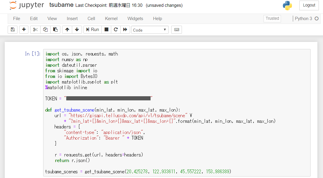
import os, json, requests, math
import numpy as np
import dateutil.parser
from skimage import io
from io import BytesIO
import matplotlib.pyplot as plt
%matplotlib inline

TOKEN = "ここには自分のアカウントのトークンを貼り付ける"

def get_tsubame_scene(min_lat, min_lon, max_lat, max_lon):
    url = "https://gisapi.tellusxdp.com/api/v1/tsubame/scene"
        + "?min_lat={}&min_lon={}&max_lat={}&max_lon={}".format(min_lat, min_lon, max_lat, max_lon)
    headers = {
        "content-type": "application/json",
        "Authorization": "Bearer " + TOKEN
    }

    r = requests.get(url, headers=headers)
    return r.json()

tsubame_scenes = get_tsubame_scene(20.425278, 122.933611, 45.557222, 153.986389)
Please get a token from API access setup (login required) on Mypage.
Click on “Run” to execute the code, and you can obtain all the scenes of images from “TSUBAME” that are available at that time.
print(len(tsubame_scenes))
At the time of writing, we could obtain 35 scenes.
print(tsubame_scenes[0])
io.imshow(io.imread(tsubame_scenes[0]['thumbs_url']))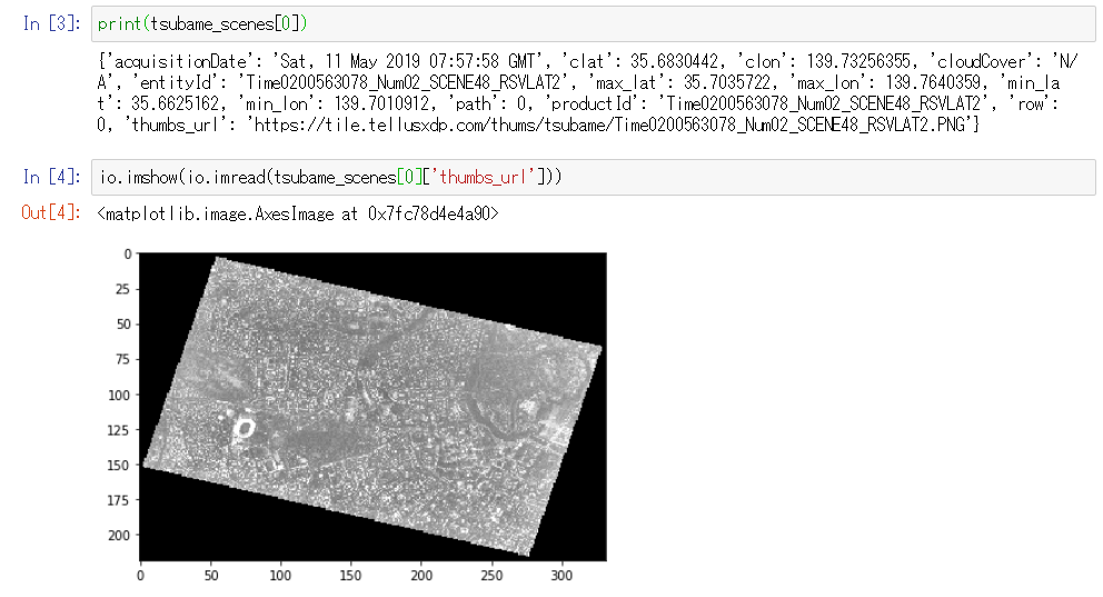
(2)Classify scenes by observation area
From April 2, “TSUBAME” had been observing two fixed points around “Akasaka Guest House” and around “Koishikawa” every day for about one month.
It will be useful to classify the scenes into “Akasaka Guest House” and “Koishikawa” for checking daily changes.
observation_areas = [
    {
        "name":"赤坂迎賓館",
        "lat": 35.68031,
        "lon": 139.729216
    },
    {
        "name":"小石川",
        "lat": 35.719582,
        "lon": 139.744686
    }
]

def classify(areas, scenes):
    result = [[] for i in range(len(areas))]

    for scene in scenes:
        dists = [np.linalg.norm(np.array([scene["clat"], scene["clon"]]) - np.array([area["lat"], area["lon"]])) for area in areas]
        result[np.argmin(dists)].append(scene)

    for i in range(len(result)):
        result[i] = sorted(result[i], key=lambda scene: dateutil.parser.parse(scene["acquisitionDate"]))
    return result

classified_scenes = classify(observation_areas, tsubame_scenes)

akasaka_scenes = classified_scenes[0]
koishigawa_scenes = classified_scenes[1]

print(len(akasaka_scenes))
print(len(koishigawa_scenes))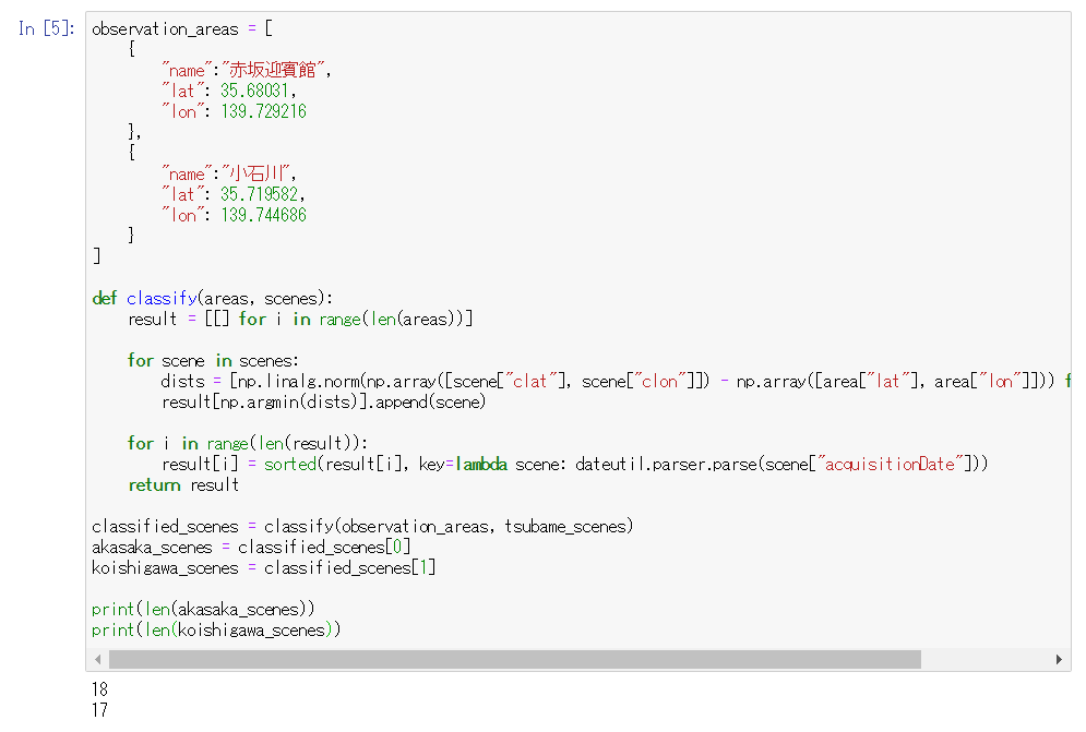
This function calculates the distance between the latitude/longitude (clat, clon) of the scene center and the representative coordinates of the observation area, and classifies each scene into a closer observation area.
At the time of writing, there were 18 scenes around “Akasaka Guest House” and 17 around “Koishikawa.”
And the classified scenes are sorted by observation date.
for scene in akasaka_scenes:
    print(scene["acquisitionDate"])
(3)Find a message displayed in the Meiji Jingu Stadium
During the “TSUBAME” observation period, JAXA and the baseball team “Tokyo Yakult Swallows” were carrying out a collaboration project to create a message by displaying large letters on the outfield seats of the Jingu Stadium for several days.
Let’s check this message on Jupyter Notebook.
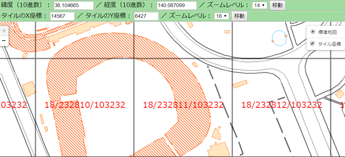
The letters were displayed on the right-field seats of the stadium, and the map tile coordinates are z=18, x=232811, and y=103232.
def get_tsubame_image(scene_id, zoom, xtile, ytile):
    url = " https://gisapi.tellusxdp.com/tsubame/{}/{}/{}/{}.png".format(scene_id, zoom, xtile, ytile)
    headers = {
        "Authorization": "Bearer " + TOKEN
    }

    r = requests.get(url, headers=headers)
    return io.imread(BytesIO(r.content))

io.imshow(get_tsubame_image(akasaka_scenes[-1]['entityId'], 18, 232811, 103232))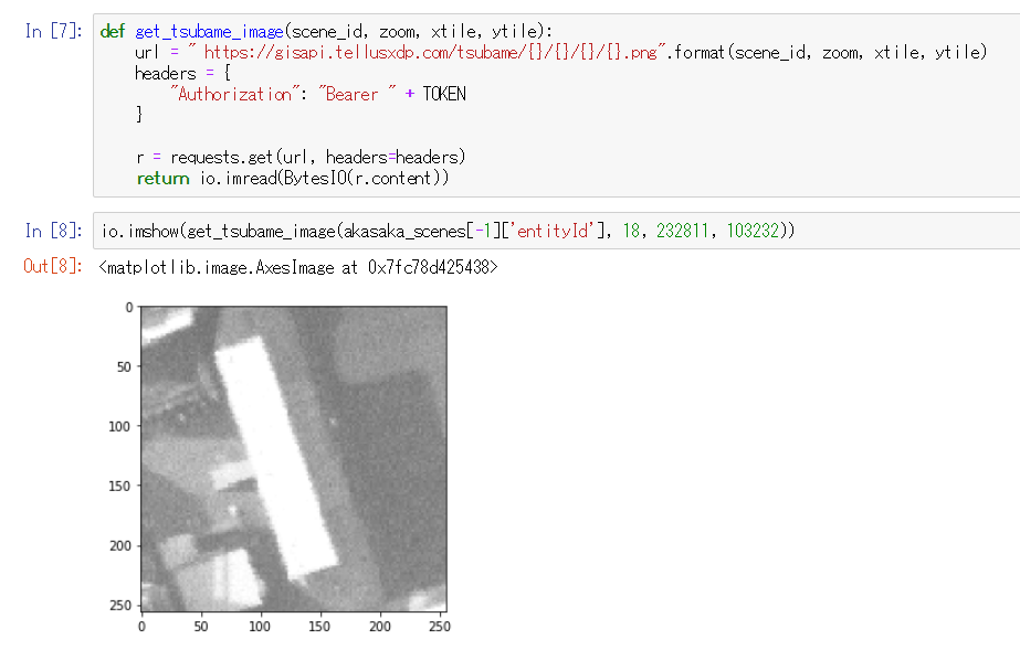
However, when we actually obtained the image at these coordinates, the stadium’s outfield seats did not appear in the image.
For most satellite images, an image taken at an angle to the subject will be processed and corrected as if it were taken from right above, but since “TSUBAME” is an engineering demonstration satellite, the distortion in this processing and correction is larger than usual, which causes a deviation from the actual point.
Therefore, even if we specify the coordinates, an image of a position deviated from the original will come out.
In this case, by shifting the coordinates toward the north to z=18, x=232811,
y=103230, we were able to obtain an image of the outfield seats of the stadium.
io.imshow(get_tsubame_image(akasaka_scenes[-1]['entityId'], 18, 232811, 103230))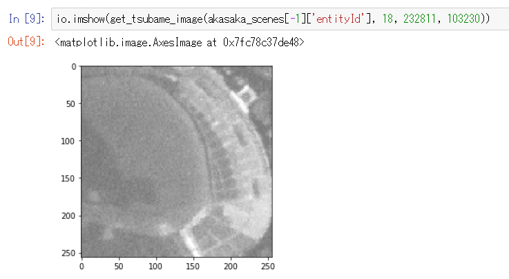
Since the amount of deviation differs according to each scene, this time, we will obtain several images around the specified coordinates, and create a function to join them into one image.
def get_tsubame_series_image(scene_id, zoom, topleft_x, topleft_y, size_x=1, size_y=1):
    img = []
    for y in range(size_y):
        row = []
        for x in range(size_x):
            row.append(get_tsubame_image(scene_id, zoom, topleft_x + x, topleft_y + y))
        img.append(np.hstack(row))
    return  np.vstack(img)
io.imshow(get_tsubame_series_image(akasaka_scenes[-1]['entityId'], 18, 232811, 103230, 2, 2))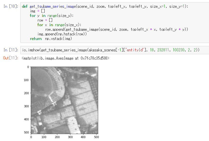
If we obtain an image of such a wide range, the right-field seats of the Jingu Stadium are within the image, even with the deviation.
The image that can be obtained through API is 256 pixels in height and width, but since this image joins four images (2×2), it is 512 pixels in height and width.
Now, let’s pick out each part around the Jingu Stadium from the previously obtained 18 scenes around “Akasaka Guest House,” and line them up.
def make_grid_image(images, col):
    img = []
    for i in range(math.ceil(len(images)/col)):
        row = []
        for j in range(col):
            index = i*col + j
            if index < len(images):
                row.append(images[index])
            else:
                row.append(np.ones_like(imgs[0])*255)
        img.append(np.hstack(row))
    return np.vstack(img)

imgs = [get_tsubame_series_image(scene['entityId'], 18, 232811, 103230, 2, 2) for scene in akasaka_scenes]

plt.rcParams['figure.figsize'] = (12, 12) #表示サイズを拡大
io.imshow(make_grid_image(imgs, 4))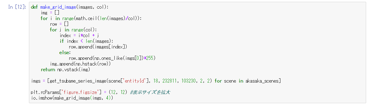
Find images with letters displayed on the outfield seats from these.
If it is too small to look for,
plt.rcParams['figure.figsize'] = (12, 12)enter a bigger number for this part.
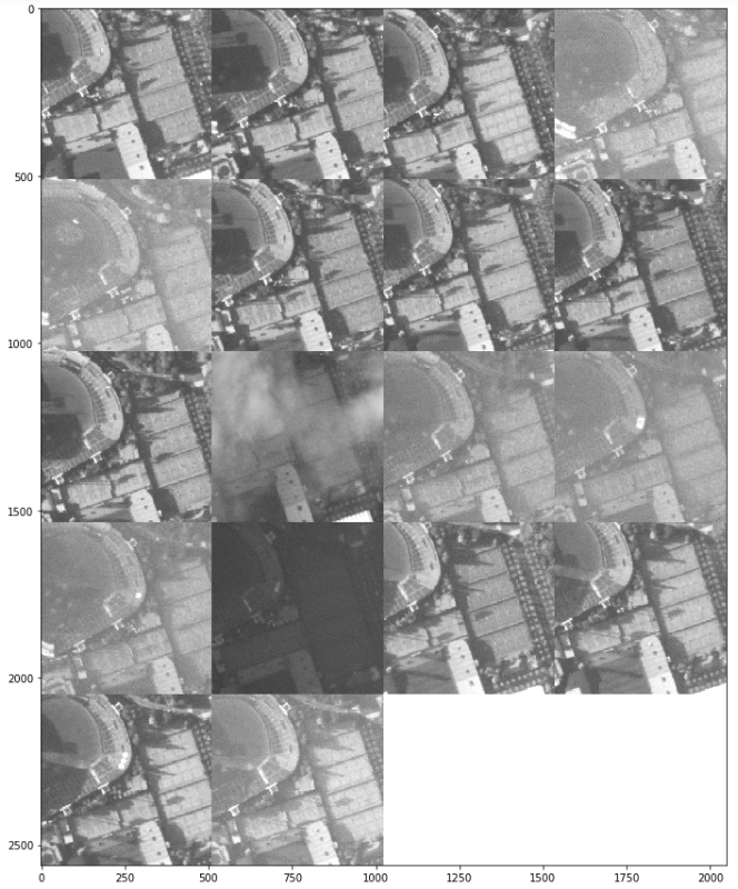
Can you see the letters on the 13th, 14th, and 17th images?
Let’s pick out just these three images and line them up.
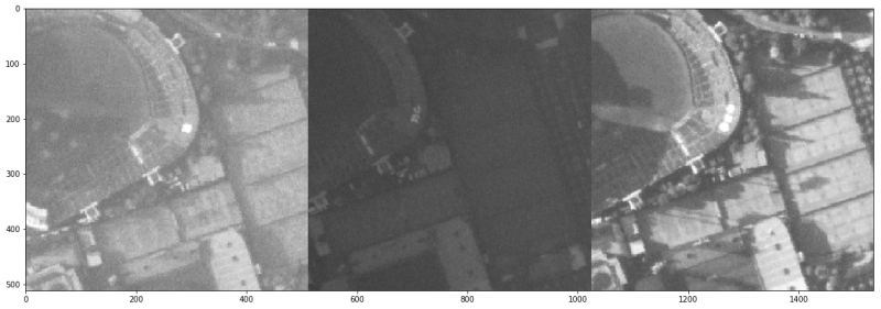
Although some images are blurred, we were able to read the message of “祝つばめ50 (Congratulations Swallows for your 50th anniversary).”
That’s how to use Jupyter Notebook on Tellus to obtain a high-resolution image from “TSUBAME” (SLATS).
There are so many points other than the Jingu Stadium that are changing day by day in Tokyo so let’s observe how this city changes.