[How to Use Tellus from Scratch] Clip area from satellite data specified in the GeoJSON format on Jupyter Notebook
Here, we will show you how to clip an area specified in GeoJSON format from satellite data obtained on Jupyter on Tellus. See "Tellusの開発環境でAPI引っ張ってみた (Use Tellus API from the development environment)" for how to use Jupyter Notebook on Tellus.
Here, we will show you how to clip an area specified in GeoJSON format from satellite data obtained on Jupyter on Tellus.
See “Tellusの開発環境でAPI引っ張ってみた (Use Tellus API from the development environment)” for how to use Jupyter Notebook on Tellus.
1. Specify the area to clip
Previously we showed an example from Sorabatake, on how to get and analyze satellite data (【ゼロからのTellusの使い方】Jupyter NotebookでAVNIR-2/ALOSの光学画像から緑地割合算出 [Beginner’s guide to Tellus — Calculate proportion of vegetation in optical image of AVNIR-2/ALOS on Jupyter Notebook]).
In that article, an entire image was analyzed. However, there are times you want to clip an area to analyze rather than using the entire image.
Here are example cases of agricultural data:
・Compare the growth of rice between point A and B in a rice paddy to find suitable condition to cultivate.
・Compare the present and past crop growth at the same point in a field to estimate the yield of the year.
・Vector data that contains location information is needed to specify the area to clip.
In a simple example, we draw a shape over the area to clip while viewing the map or satellite image. Then, we use the area for some analytical purpose.
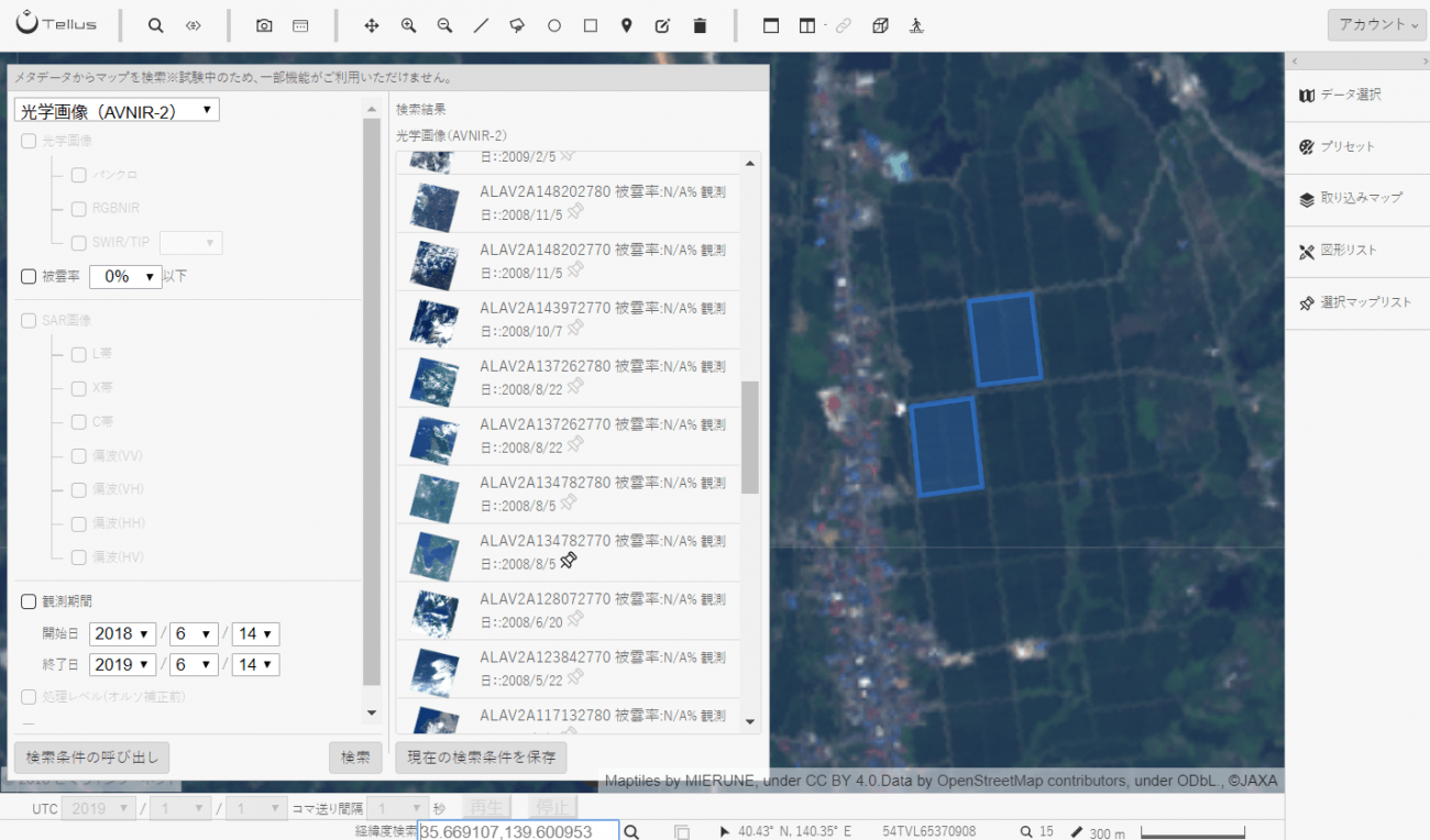
First, choose from satellite data, the area from which you want to clip.
In this example, we clip an area around Harumi, Tokyo from AVNIR-2 data.
Place Takeshiba pier in the center of the screen and click “メタデータ検索 (Search by metadata)”.
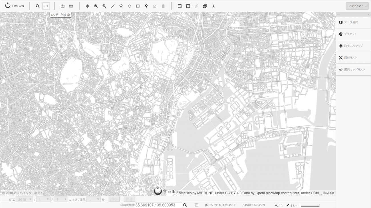
Choose “光学画像 (AVNIR-2) (Optical images [AVNIR-2])” in the opened panel and click “検索 (Search)”. Observation data items will be listed each with its range displayed.
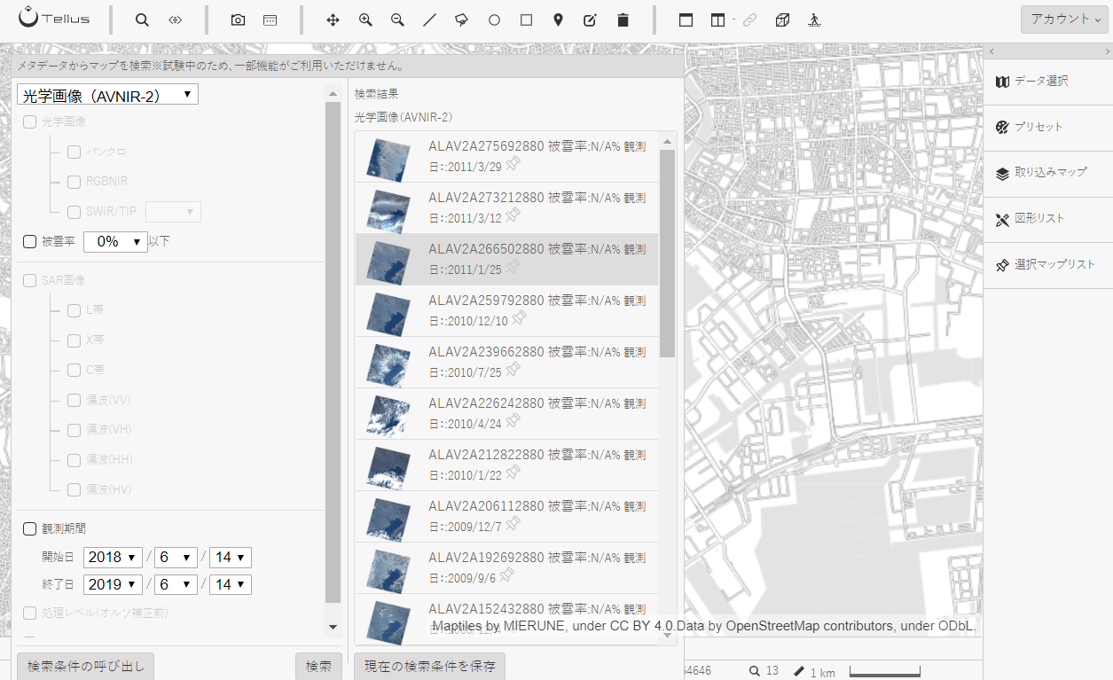
Choose the observation data item you want to use from the list to display it on the OS (in this example, ALAV2A266502880 is chosen).
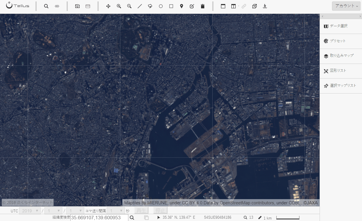
Next, draw a shape over the area to clip.
This time, we clip the reclaimed land around Harumi.
Click “多角形を追加 (Add a polygon)” among the icons at the top of the screen to draw a shape that fits the shape of the reclaimed land.
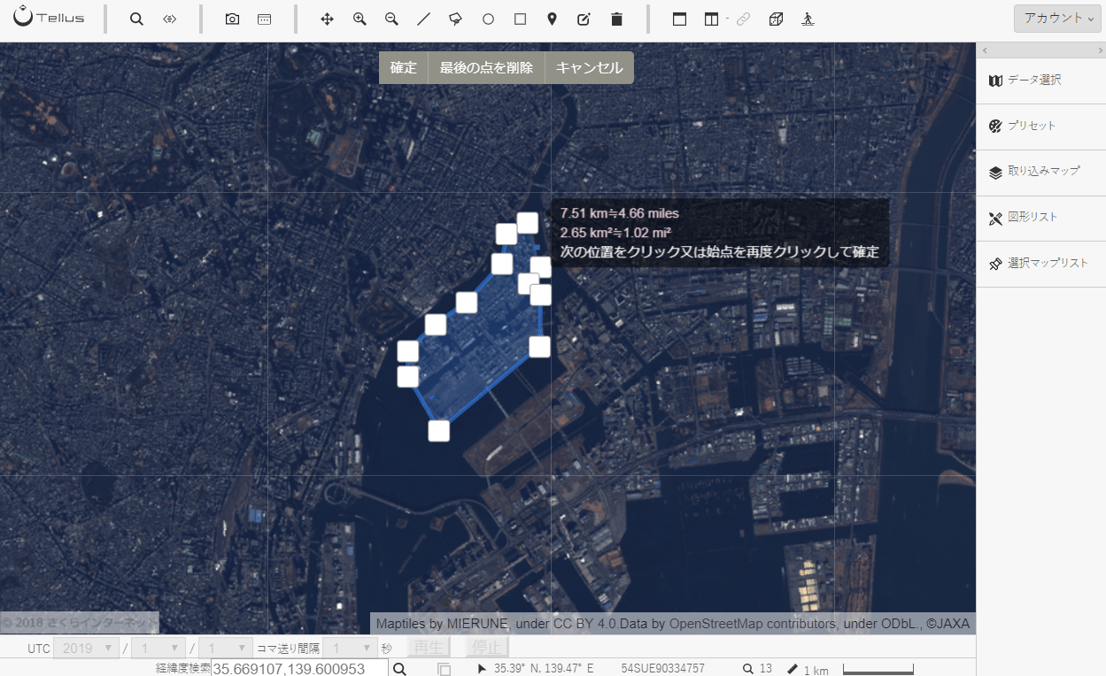
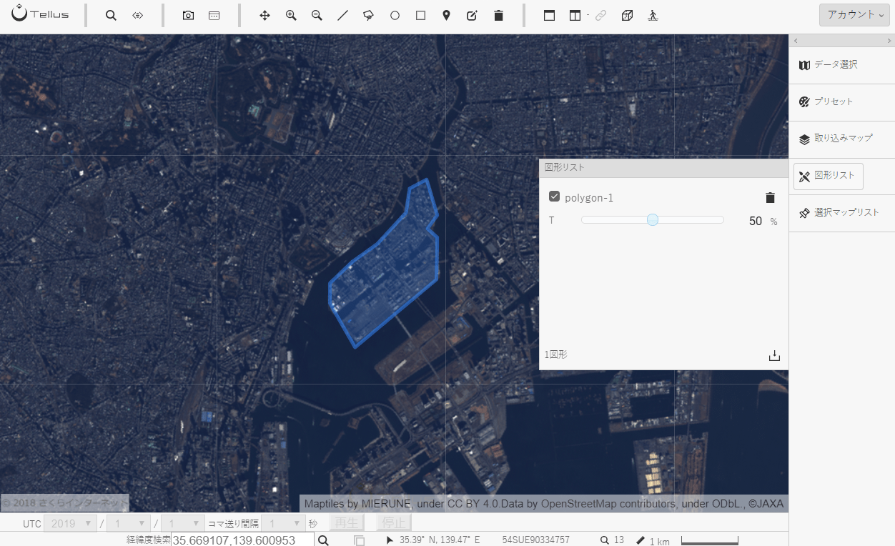
Complete it by properly enclosing it. The created shape can be viewed in the “図形リスト (Shape list)” at the right of the screen.
This time, it’s stored as “polygon-1”.
2. Get the satellite data and GeoJSON data of the area to clip on Jupyter Notebook
Get the satellite data you want to analyze and the created shape on Jupyter Notebook.
Run the code below to get the AVNIR-2 data using the scene ID (ALAV2A266502880 in this example) and tile coordinates.
import os, json, requests, math
import numpy as np
from skimage import io
from io import BytesIO
from skimage.draw import polygon
%matplotlib inline
TOKEN = "ここには自分のアカウントのトークンを貼り付ける"
def get_AVNIR_SCENEID(scene_id):
url = "https://gisapi.tellusxdp.com/api/v1/av2ori/get_scene/{}".format(scene_id)
headers = {
"Authorization": "Bearer " + TOKEN
}
r = requests.get( url, headers=headers )
return r.json()
def get_AVNIR_image(rspid, sceneid, zoom, xtile, ytile, opacity=1, r=3, g=2, b=1, rdepth=1, gdepth=1, bdepth=1, preset=None):
url = "https://gisapi.tellusxdp.com/av2ori/{}/{}/{}/{}/{}.png?opacity={}&r={}&g={}&b={}&rdepth={}&gdepth={}&bdepth={}".format(rspid, sceneid, zoom, xtile, ytile, opacity, r, g, b, rdepth, gdepth, bdepth)
headers = {
"Authorization": "Bearer " + TOKEN
}
url = "https://gisapi.tellusxdp.com/av2ori/{}/{}/{}/{}/{}.png".format(rspid, sceneid, zoom, xtile, ytile)
payload = { "preset": preset, "opacity": opacity, "r": r, "g": g, "b": b, "rdepth": rdepth, "gdepth": gdepth, "bdepth": bdepth }
r = requests.get( url, params=payload, headers=headers )
return io.imread(BytesIO(r.content))
sceneid1 = "ALAV2A266502880" #取得したいシーンID
tile1 = {"x": 7276, "y": 3226, "z": 13} #取得したい地点のタイル座標
scene1 = get_AVNIR_SCENEID(sceneid1)
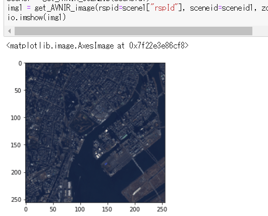
img1 = get_AVNIR_image(rspid=scene1["rspId"], sceneid=sceneid1, zoom=tile1["z"], xtile=tile1["x"], ytile=tile1["y"])
io.imshow(img1)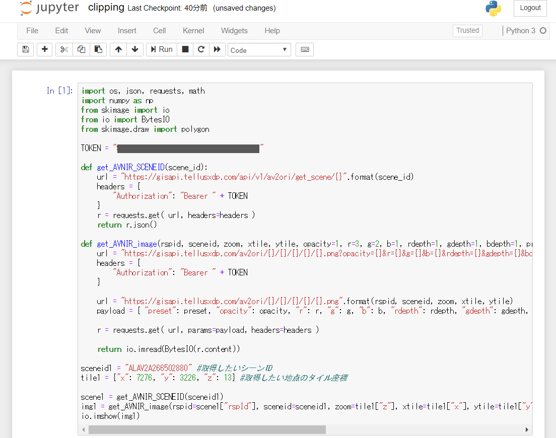
Get the token from APIアクセス設定 (API access setting) in My Page (login required).
See the API reference for more information about the API to search for scene IDs and the API to get scenes of AVNIR-2.
Run the code below to get the shape created on the OS (“polygon-1” in this example).
See Beginner’s guide for Tellus — Save and get spatial data (GeoJSON) on Jupyter Notebook for more information about how to get shapes using the API.
def get_shape_geojson_by_name(name):
    URL = "https://api.tellusxdp.com/v1/shapes"
    headers = {
        "Authorization": "Bearer " + TOKEN
    }

    r = requests.get(URL , headers=headers)
    shapes = r.json()
    shape = next((shape for shape in shapes["items"] if shape["name"]==name) ,None)
    return json.loads(shape["data"])


shapename1 = "polygon-1"
shape1 = get_shape_geojson_by_name(shapename1)
print(shape1)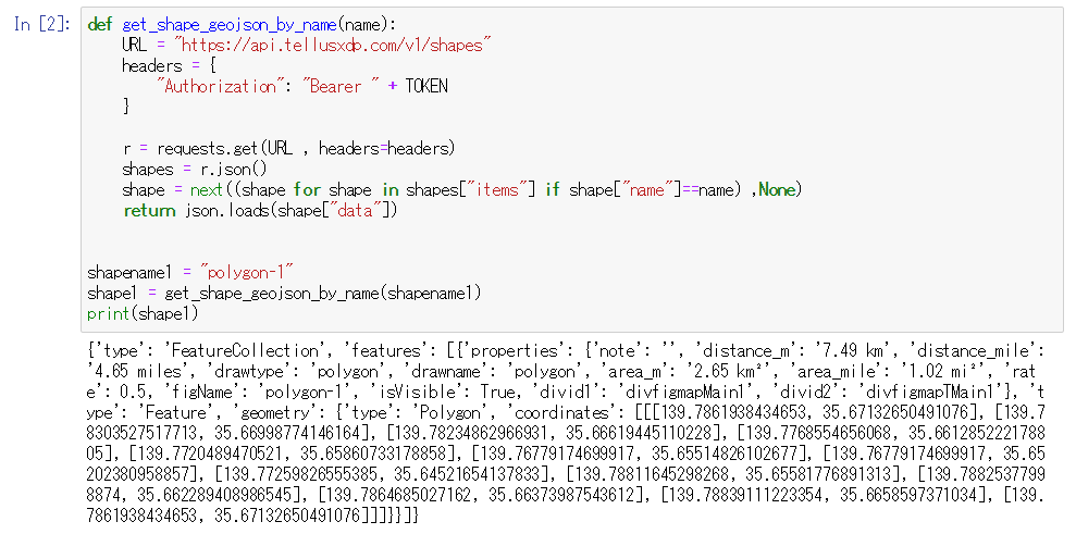
3. Clipping
Now, clip the area from the satellite image using the obtained shape.
Apexes of the shape are represented by latitudes and longitudes. You need to convert them into pixel coordinates.
Then, use the polygon function in the image processing library skimage to generate an array where pixels within the area are assigned 1 and others 0.
def get_tile_bbox(xtile, ytile, zoom):
    """
    タイル座標からバウンダリボックスを取得
    https://tools.ietf.org/html/rfc7946#section-5
    """
    def num2deg(xtile, ytile, zoom):
        # https://wiki.openstreetmap.org/wiki/Slippy_map_tilenames#Python
        n = 2.0 ** zoom
        lon_deg = xtile / n * 360.0 - 180.0
        lat_rad = math.atan(math.sinh(math.pi * (1 - 2 * ytile / n)))
        lat_deg = math.degrees(lat_rad)
        return (lon_deg, lat_deg)

    right_top = num2deg(xtile + 1, ytile, zoom)
    left_bottom = num2deg(xtile, ytile + 1, zoom)
    return (left_bottom[0], left_bottom[1], right_top[0], right_top[1])


def get_polygon_image(points, bbox, imgsize):
    def world2pixel(bbox, size, lon, lat):
        """
        経度緯度をピクセル座標に変換
        """
        dist = ((bbox[2] - bbox[0])/size[0], (bbox[3] - bbox[1])/size[1])
        pixel = (int((lon - bbox[0]) / dist[0]), int((bbox[3] - lat) / dist[1]))
        return pixel

    pixels = []
    for p in points:
        pixels.append(world2pixel(bbox, (imgsize["width"], imgsize["height"]), p[0], p[1]))
    pixels = np.array(pixels)

    poly = np.ones((imgsize["height"], imgsize["width"]), dtype=np.uint8)
    rr, cc = polygon(pixels[:, 1], pixels[:, 0], poly.shape)
    poly[rr, cc] = 0
    return poly

points1 = shape1["features"][0]["geometry"]["coordinates"][0]
bbox1 = get_tile_bbox(tile1["x"], tile1["y"], tile1["z"])
pxsize1 = {"width": img1.shape[1], "height": img1.shape[0]}

mask1 = get_polygon_image(points1, bbox1,pxsize1)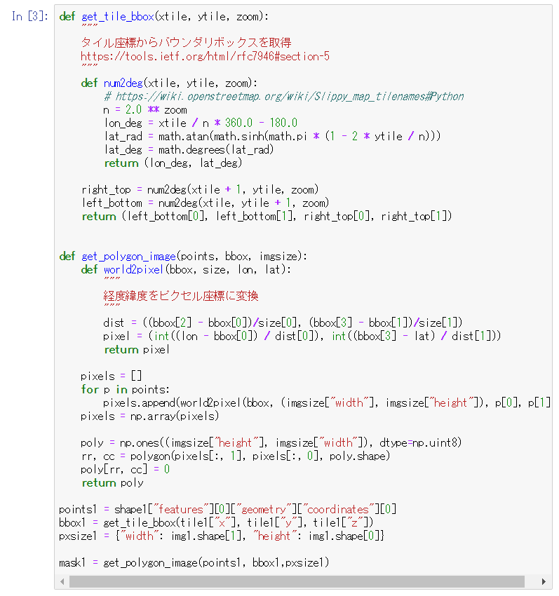
If you visualize the generated array, it looks as shown below.
io.imshow(mask1)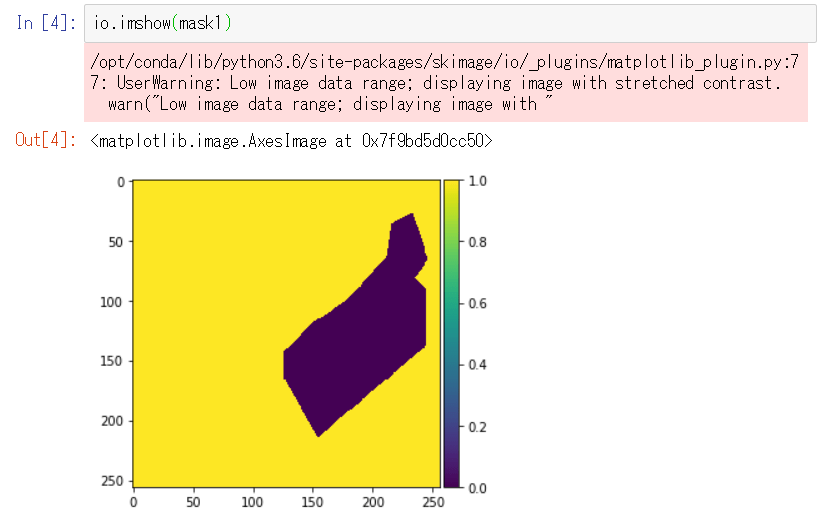
You may get warnings, but you can ignore them.
Use this image of the shape and the choose function in numpy to clip the area from the satellite image.
def clip(img, mask):
    base = img.transpose(2, 0, 1)[:3,:]
    cliped = np.choose(mask, (base, 0)).astype(np.uint8)
    return cliped.transpose(1, 2, 0)

cliped1 = clip(img1, mask1)
io.imshow(cliped1)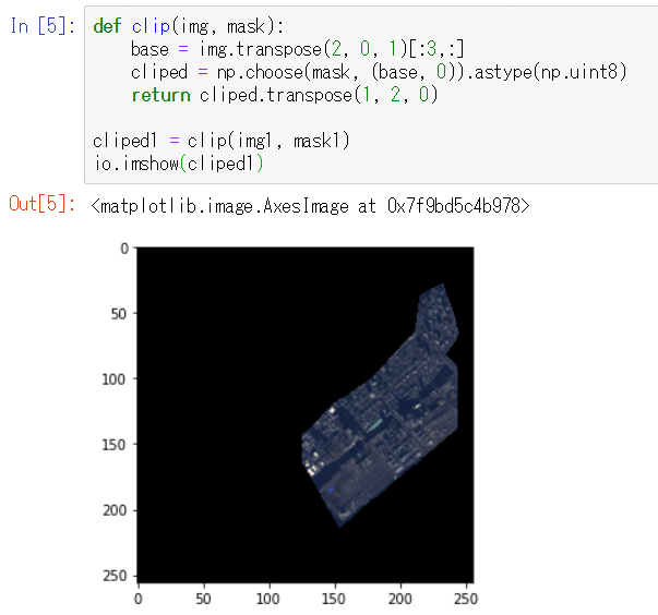
The area is clipped in the shape of the reclaimed land.
4. Compare two points
Now that area is clipped from satellite data, let’s use it for analysis.
As an example, we will compare rice growth between two points in a rice paddy using NDVI.
*See 【ゼロからのTellusの使い方】Jupyter NotebookでAVNIR-2/ALOSの光学画像から緑地割合算出 (Beginner’s guide to Tellus — Calculate proportion of vegetation in optical image of AVNIR-2/ALOS on Jupyter Notebook) for how to calculate the portion of the vegetation in an image using NDVI.
Choose points for comparison and create shapes over them.
The location is around (40.73440677988237,140.59194660134384).
sceneid2 = "ALAV2A134782770" #取得したいシーンID
tile2 = {"x": 14590, "y": 6158, "z": 14} #取得したい地点のタイル座標

scene2 = get_AVNIR_SCENEID(sceneid2)
img2 = get_AVNIR_image(rspid=scene2["rspId"], sceneid=sceneid2, zoom=tile2["z"], xtile=tile2["x"], ytile=tile2["y"], preset="ndvi")
io.imshow(img2)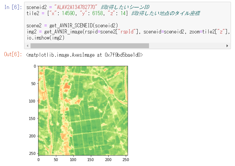
bbox2 = get_tile_bbox(tile2["x"], tile2["y"], tile2["z"])
pxsize2 = {"width": img2.shape[1], "height": img2.shape[0]}

shapename2_1 = "polygon-2" #自分で作った図形の名前に変更する
shape2_1 = get_shape_geojson_by_name(shapename2_1)
points2_1 = shape2_1["features"][0]["geometry"]["coordinates"][0]
mask2_1 = get_polygon_image(points2_1, bbox2, pxsize2)

shapename2_2 = "polygon-3" #自分で作った図形の名前に変更する
shape2_2 = get_shape_geojson_by_name(shapename2_2)
points2_2 = shape2_2["features"][0]["geometry"]["coordinates"][0]
mask2_2 = get_polygon_image(points2_2, bbox2, pxsize2)


cliped2_1 = clip(img2, mask2_1)
cliped2_2 = clip(img2, mask2_2)
io.imshow(np.hstack((cliped2_1, cliped2_2)))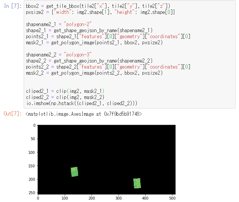
import cv2

def filter_green(img):
    green_min = np.array([55,0,0])
    green_max = np.array([75,255,255])
    # OpenCVで扱うために色順をRGB(RGBA)からBGRに入れ替える
    cv_bgr = cv2.cvtColor(img, cv2.COLOR_RGBA2BGR)
    # BGRからHSVに変換
    cv_hsv = cv2.cvtColor(cv_bgr, cv2.COLOR_BGR2HSV)

    # 指定した範囲の色以外を黒に変換する
    mask = cv2.inRange(cv_hsv, green_min, green_max)
    masked_img = cv2.bitwise_and(cv_bgr, cv_bgr, mask=mask)

    # 得られた画像の色順をBGRからRGBに戻す
    return cv2.cvtColor(masked_img, cv2.COLOR_BGR2RGB)

filtered_img2_1 = filter_green(cliped2_1)
filtered_img2_2 = filter_green(cliped2_2)
io.imshow(np.hstack((filtered_img2_1, filtered_img2_2)))

def count_not_black(img):
    return len(np.nonzero(img.ravel())[0])

# 切り出した領域内の緑色のピクセルの割合
print("領域1: {:.2f}%".format(count_not_black(filtered_img2_1) / count_not_black(cliped2_1) * 100))
print("領域2: {:.2f}%".format(count_not_black(filtered_img2_2) / count_not_black(cliped2_2) * 100))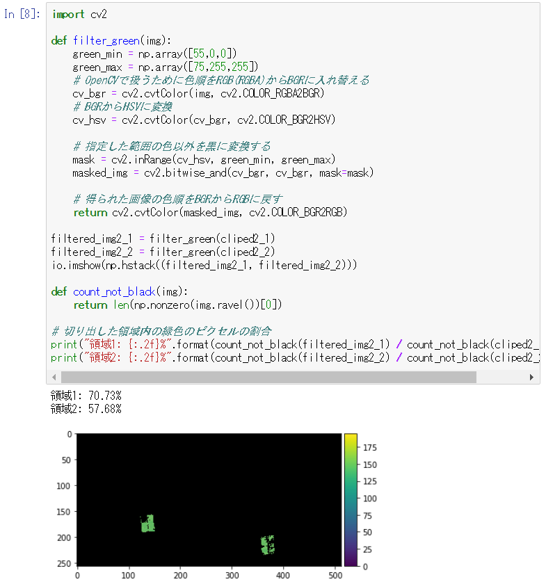
In this example analysis, rice grows better at point A than at point B (point A: about 71%, point B: about 58%).
5. Time-series comparison
You can also compare the growth in the present and the past of the chosen area points.
Choose a point for comparison and draw a shape over it.
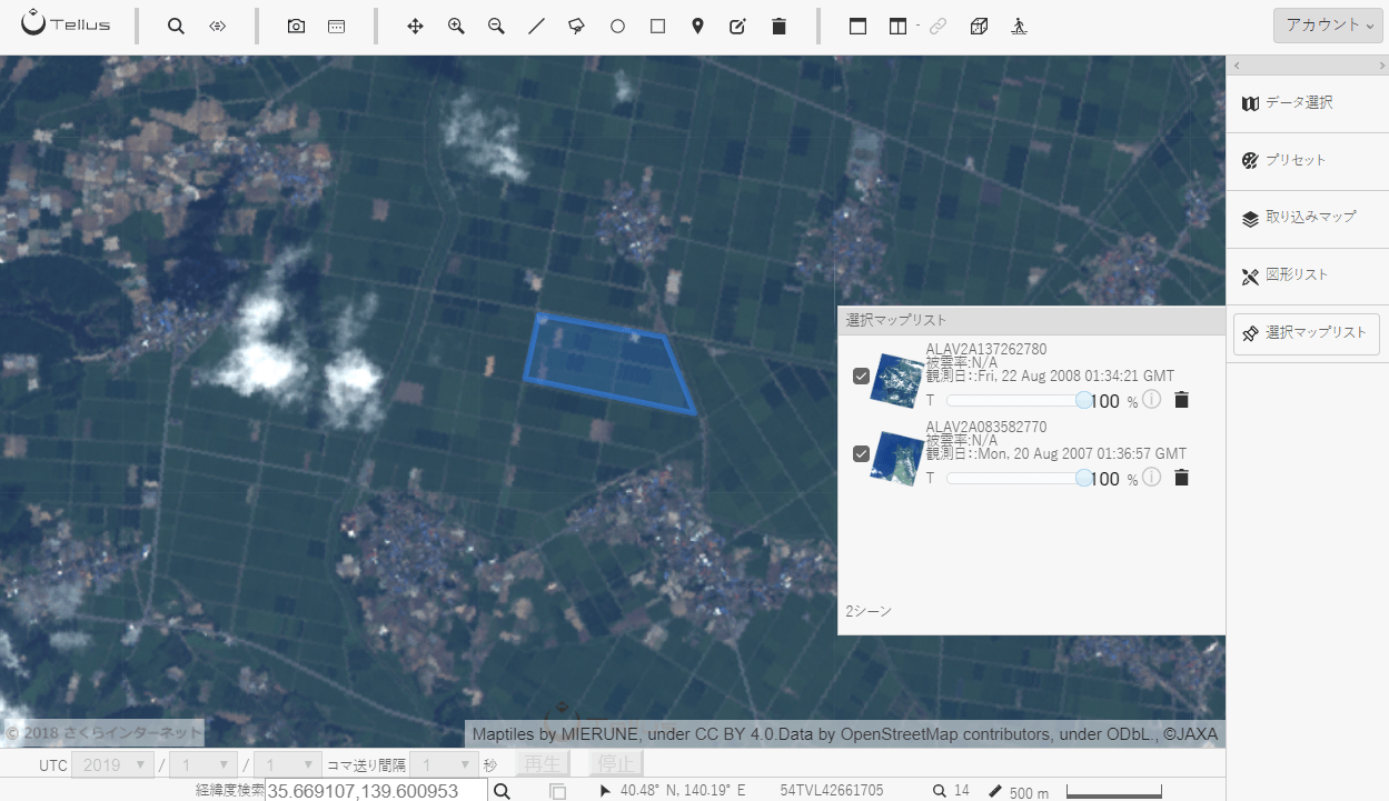
The location is around (40.8034148344062,140.3250432014465).
tile3 = {"x": 14578, "y": 6154, "z": 14} #取得したい地点のタイル座標
sceneid3_1 = "ALAV2A137262780" #取得したいシーンID
scene3_1 = get_AVNIR_SCENEID(sceneid3_1)
sceneid3_2 = "ALAV2A083582770" #取得したいシーンID
scene3_2 = get_AVNIR_SCENEID(sceneid3_2)

img3_1 = get_AVNIR_image(rspid=scene3_1["rspId"], sceneid=sceneid3_1, zoom=tile3["z"], xtile=tile3["x"], ytile=tile3["y"], preset="ndvi")
img3_2 = get_AVNIR_image(rspid=scene3_2["rspId"], sceneid=sceneid3_2, zoom=tile3["z"], xtile=tile3["x"], ytile=tile3["y"], preset="ndvi")
io.imshow(np.hstack((img3_1, img3_2)))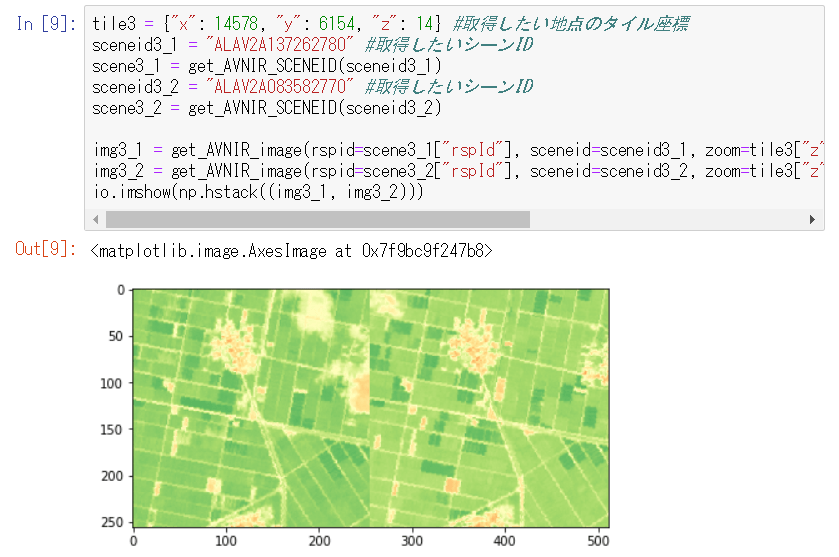
bbox3 = get_tile_bbox(tile3["x"], tile3["y"], tile3["z"])
pxsize3 = {"width": img3_1.shape[1], "height": img3_1.shape[0]}

shapename3 = "polygon-4" #自分で作った図形の名前に変更する
shape3 = get_shape_geojson_by_name(shapename3)
points3 = shape3["features"][0]["geometry"]["coordinates"][0]
mask3 = get_polygon_image(points3, bbox3, pxsize3)

cliped3_1 = clip(img3_1, mask3)
cliped3_2 = clip(img3_2, mask3)
io.imshow(np.hstack((cliped3_1, cliped3_2)))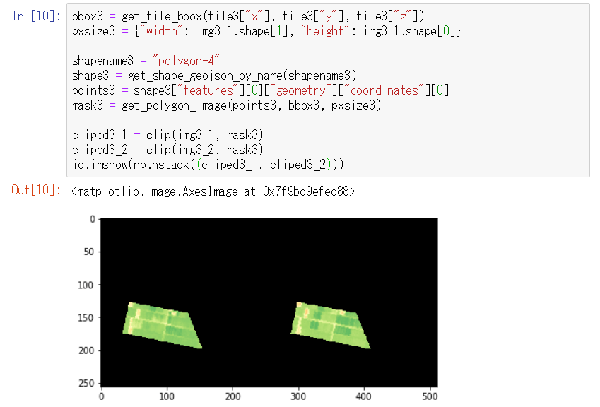
filtered_img3_1 = filter_green(cliped3_1)
filtered_img3_2 = filter_green(cliped3_2)
io.imshow(np.hstack((filtered_img3_1, filtered_img3_2)))

# 切り出した領域内の緑色のピクセルの割合
print("領域1: {:.2f}%".format(count_not_black(filtered_img3_1) / count_not_black(cliped3_1) * 100))
print("領域2: {:.2f}%".format(count_not_black(filtered_img3_2) / count_not_black(cliped3_2) * 100))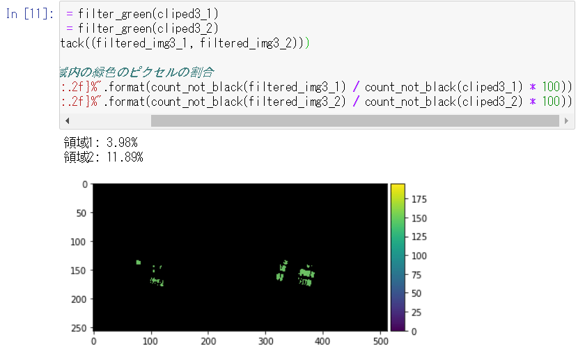
In this example analysis, rice didn’t grow as well in August 2008 as in August 2007 (2008: about 4%, 2007: about 12%). Accordingly, you can assume the yield was lower in 2008 than in 2007.
This is how to clip an area specified in the GeoJSON format from satellite data obtained from Jupyter Notebook on Tellus.
You can clip more complex shapes as long as you prepare the GeoJSON data. If you alter the code a little, you can do the same thing with vector data in other formats other than GeoJSON, such as Shapefile.
This time, we showed you two analyzed examples.
In practice, you need trial and error for selection of scenes and points (presence of clouds, observation direction and observation time), adjustment to thresholds (range of vegetation) and other things, but try to conduct data analysis using combined satellite and spatial data with reference to this article.