We would like to introduce how to extract green space from the optical image using AVNIR-2/ALOS data on Tellus.

In this article, we will reveal how to extract green space from AVNIR-2/ALOS optical image using Jupyter Notebook on Tellus.

Please refer to “API available in the Developing Environment of Tellus” for how to use Jupyter Notebook on Tellus.

(1) Obtain NDVI image using API of AVNIR-2

In the previous article, “[How to Use Tellus from Scratch] Obtain AVNIR-2/ALOS Optical Image on Jupyter Notebook ,” we have introduced how to use the optical image obtained by AVNIR-2/ALOS on Tellus Jupyter Notebook.

This time, we are using True Color composite and Natural Color composite, but AVNIR-2 data could also be used in many other ways.

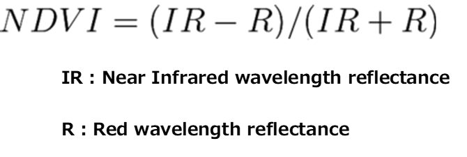
Let’s obtain the image that describes vegetation activity (NDVI), which measures the amount of growing vegetation, in colors.

Plants generally tend to absorb red wavelength lights the best, while they reflect near-infrared wavelength lights as well.

NDVI takes advantage of its nature.

import os, json, requests, math
import numpy as np
import cv2
from skimage import io
from io import BytesIO
import matplotlib.pyplot as plt
%matplotlib inline

TOKEN = "ここには自分のアカウントのトークンを貼り付ける"

def get_AVNIR_image(zoom, xtile, ytile, opacity=1, r=3, g=2, b=1, rdepth=1, gdepth=1, bdepth=1, preset=None):
    url = "https://gisapi.tellusxdp.com/blend/{}/{}/{}.png?opacity={}&r={}&g={}&b={}&rdepth={}&gdepth={}&bdepth={}".format(zoom, xtile, ytile, opacity, r, g, b, rdepth, gdepth, bdepth) 
    if preset is not None:
        url += '&preset='+preset
    headers = {
        "content-type": "application/json",
        "Authorization": "Bearer " + TOKEN
    }
    r = requests.get(url, headers=headers)
    return io.imread(BytesIO(r.content))

true_img1 = get_AVNIR_image(zoom=13,xtile=7276,ytile=3226)
ndvi_img1 = get_AVNIR_image(zoom=13,xtile=7276,ytile=3226,preset='ndvi')
io.imshow(np.hstack((true_img1, ndvi_img1)))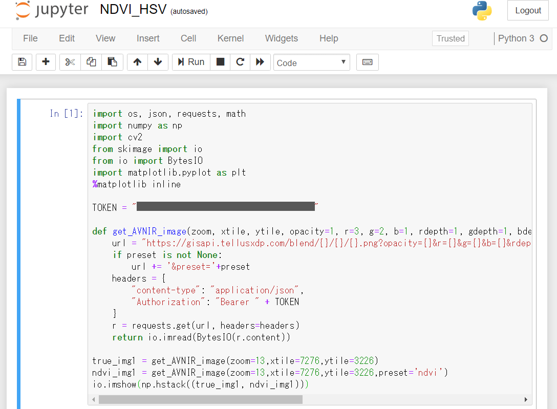

Click “Run,” and the optical image around Tsukiji, Tokyo will be displayed.

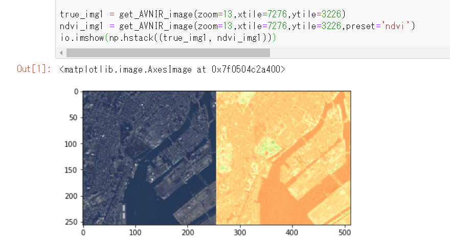
In NDVI composite, the healthy vegetation is colored in green and the poor vegetation in red.

That is why the locations around Hama-rikyu Garden in the center, Shiba Park on the left, and Hibiya Park on the top left appear to glow yellow-green in NDVI composite. (*It might be a bit difficult to tell the color boundaries.)

(2) HSV Conversion

You can extract the green space just by extracting yellow and green parts in NDVI composite. HSV conversion is often used for color extraction.

While RGB uses the information of red, green, and blue to display the color, HSV uses hue (types of colors), saturation (clarity), and value (brightness) instead.

*Please search “HSV color space” for more information.

Let’s use an image processing library called OpenCV for color conversion and extraction. Hue ranges from 0 to 180 in OpenCV.

Saturation and value range from 0 to 255, respectively .

def masking(img, hsv_min, hsv_max):
    # OpenCVで扱うために色順をRGB(RGBA)からBGRに入れ替える
    cv_bgr = cv2.cvtColor(img, cv2.COLOR_RGBA2BGR) 
    # BGRからHSVに変換
    cv_hsv = cv2.cvtColor(cv_bgr, cv2.COLOR_BGR2HSV)
    
    # 指定した範囲の色以外を黒に変換する
    mask = cv2.inRange(cv_hsv, hsv_min, hsv_max)
    masked_img = cv2.bitwise_and(cv_bgr, cv_bgr, mask=mask)

    # 指定した範囲の色の割合
    rate = len(np.where(mask.ravel()!=0)[0])/len(mask.ravel())

    # 得られた画像の色順をBGRからRGBに戻す
    return cv2.cvtColor(masked_img, cv2.COLOR_BGR2RGB), rate


green_min = np.array([25,0,0]) 
green_max = np.array([75,255,255])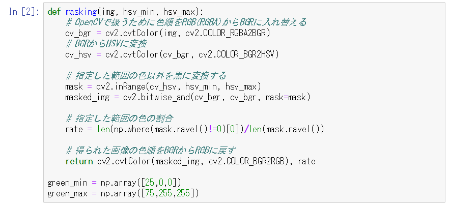 

This function is to extract only the yellow and green parts. This time, we will extract the hue from 25 to 75.

Now, pass the NDVI composite image to the function and display the result.

masked_img1, rate = masking(ndvi_img1, green_min, green_max)
io.imshow(masked_img1)
print(rate)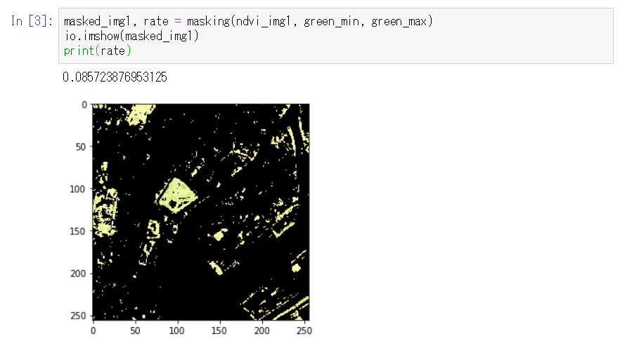

Only the yellow-green parts are extracted, which made vegetation in Hama-rikyu Garden, Shiba Park, Hibiya Park, and the landfill seawall clear.

Also, we can see that the percentage of vegetation in this image is about 9% (0.085723……).

(3) Look at the image of a suburban area

Let’s see what kind of color the suburban area will be compared to central Tokyo.

true_img2 = get_AVNIR_image(zoom=13,xtile=7253,ytile=3230)
io.imshow(true_img2)

These are the coordinates around Lake Kawaguchi at the same zooming factor

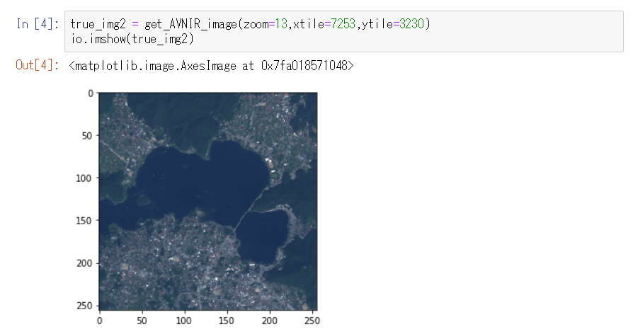
You can clearly see the border between the lake in the center and surrounding residential area or mountain area covered with trees, even in True Color composite.

Let’s obtain NDVI composite image of this location as before, and extract the vegetation area.

ndvi_img2 = get_AVNIR_image(zoom=13,xtile=7253,ytile=3230,preset='ndvi')
io.imshow(masking(ndvi_img2, green_min, green_max))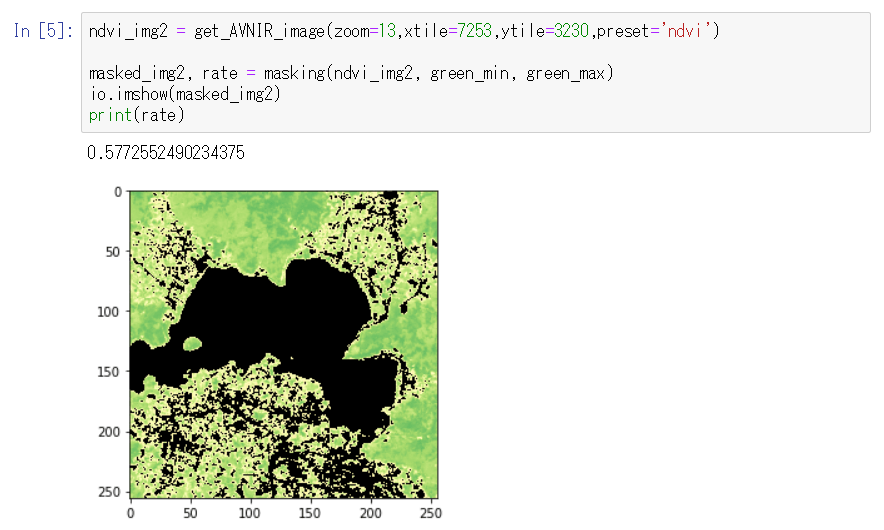

There are many dark green parts compared to Hama-rikyu Garden and its surrounding area. As expected, the vegetation is activated in the suburban area, where we can have a glance that it is actively growing.

The residential area is mottled in yellow-green.

It is because fields and homestead woodland scattered across the residential area are extracted, which is the big difference from central Tokyo where most of the land except the park is filtered black.

The percentage of the vegetation in the image is about 58%, which shows the richness in nature not only from our sense but also from the figure compared to about 9% in central Tokyo.

The above explains how to extract green space from AVNIR-2/ALOS optical image and calculate the percentage of the vegetation in the image on Jupyter Notebook.

This extraction process is just an example.

Assuming that “the yellow and green parts in NDVI composite show the green space,”

green_min = np.array([25,0,0]) 
green_max = np.array([75,255,255]) 

we have extracted the image setting the lower limit of hue to 25, and the upper limit to 75, but we need to adjust these values to improve the accuracy.

Moreover, there might be more effective extraction conditions other than using NDVI composite and HSV conversion.

Various optimal conditions can be extracted depends on your objectives, contents, and accuracy. This is the highlight of image processing but also as its difficult part.

It would be helpful to examine extraction conditions using machine learning. Starting with green space extraction, please explore how to use more advanced satellite data.