What is a satellites’ final task? The achievements of a decommissioned Super Low Altitude Test Satellite (SLATS)
Where do retired artificial satellites go when they completed their duties in space? The operation of Super Low Altitude Test Satellite (SLATS) was finalized on October 1, 2019. In this article, we will explain SLATS last job and how to interpret its observation data.
The JAXA’s Super Low Altitude Test Satellite (SLATS) finished its operation on October 1, 2019.
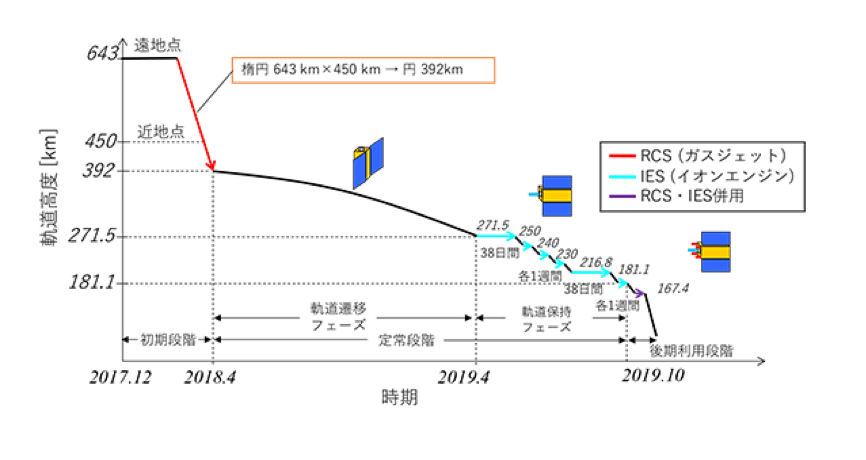
As explained in Super Low Altitude Test Satellite (SLATS): The Challenges and Expectations on Super Low Altitude Orbit, SLATS was an engineering test satellite orbiting at a super low altitude of 200 kilometers above the Earth.
In this article, we will explain the decommissioning of a satellite and how to interpret SLATS’ observation data.
What is the last job of a satellite?
Many of the earth observation satellites are going around similar trajectories according to their types. For this reason, decommissioned satellites are required to deorbit as soon as possible to avoid collisions with other satellites.
Deorbit means, for example, in the case of low-earth-orbit satellites, to move out of 400-600 kilometers above the Earth to a lower orbit. They eventually penetrate into the Earth’s atmosphere and burn up.
In addition, as the range of frequencies available to satellites is limited, decommissioned satellites need to stop using radio waves and shut down their communication devices not to occupy the frequency band unnecessarily.
If we were to liken the above to mobile phones, once you no longer need a phone number, you should terminate the contract instead of keeping it so that others can use the number you no longer need.
In short, earth observation satellites need to 1) leave the orbit and 2) stop using radio waves (shut the power off) as their last job.
Since SLATS ended up orbiting at a very low altitude, about 200 kilometers above the Earth, it seems to have penetrated the atmosphere promptly after stopping the use of radio waves to then burn up.
SLATS has provided 267 scenes at 56 spots on Tellus
SLATS has observed various spots in both Japan and the world for over 6 months. Tellus added new data on October 23, 2019, providing observed data at 56 spots (267 scenes).
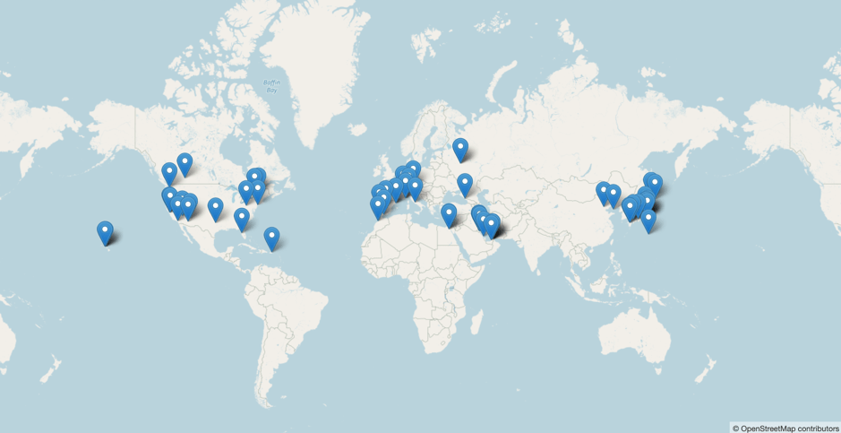
Now we are going to see how the surface of the Earth observed by SLATS looks like using Jupyter Lab (You can also check the scenes observed by SLATS on Tellus. Import GeoJSON of the observation spot and perform a metasearch within the range of the pinned spot.)
Please refer to “API available in the developing environment of Tellus” for how to use Jupyter Lab (Jupyter Notebook) on Tellus.
import os, json, requests
from skimage import io
from io import BytesIO
%matplotlib inline


TOKEN = 'ここには自分のアカウントのトークンを貼り付ける'

def search_tsubame_scenes(min_lon, min_lat, max_lon, max_lat, v='', debug=False):
    """
    経度緯度の範囲でシーンを取得

    Parameters
    ----------
    min_lon : number
        シーン取得範囲の最小経度(-180 - 180)
    min_lat : number
        シーン取得範囲の最小緯度(-90 - 90)
    max_lon : number
        シーン取得範囲の最大経度(-180 - 180)
    max_lat : number
        シーン取得範囲の最大緯度(-90 - 90)

    Returns
    -------
    content : json
        結果

    """
    url = 'https://gisapi.tellusxdp.com/api/v1/tsubame/scene'
    headers = {
        'X-Data-Version' : str(v),
        'Authorization': 'Bearer {}'.format(TOKEN)
    }
    payload = {'min_lat': min_lat, 'min_lon': min_lon,
               'max_lat': max_lat, 'max_lon': max_lon}

    r = requests.get(url, params=payload, headers=headers)
    if r.status_code is not 200:
        raise ValueError('status error({}).'.format(r.status_code))

    if debug:
        return r.headers, r.json()
    else:
        return r.json()

def get_tsubame_scene(id, v='', debug=False):
    """
    IDからシーンを取得

    Parameters
    ----------
    id : str
        シーンID

    Returns
    -------
    content : json
        結果

    """
    url = 'https://gisapi.tellusxdp.com/api/v1/tsubame/get_scene/{}'.format(id)
    headers = {
        'X-Data-Version' : str(v),
        'Authorization': 'Bearer {}'.format(TOKEN)
    }

    r = requests.get(url, headers=headers)
    if r.status_code is not 200:
        raise ValueError('status error({}).'.format(r.status_code))

    if debug:
        return r.headers, r.json()
    else:
        return r.json()
Using the sample code above, you can obtain information of the scenes observed by SLATS.
Please refer to [How to Use Tellus from Scratch] Obtain high-resolution images from “TSUBAME” (SLATS), using Jupyter Notebook. for how to obtain images (map tiles).
Get the token from APIアクセス設定 (API access setting) in My Page (login required).
Acquisition of scenes regularly observed in four cities
SLATS periodically carried out observations in the four locations of Tokyo, Waikiki, Kuwait, and Nice (France) among other locations around the world.
In Tokyo, the observation was targeted at areas around the Guest House in Akasaka and around Koishikawa. You can obtain the scenes by narrowing the range as below.
# 赤坂迎賓館周辺
# 範囲を指定してシーン情報を取得し個数を表示
tokyo_scenes1 = search_tsubame_scenes(139.72, 35.67, 139.73, 35.68)
print(len(tokyo_scenes1))

# 代表的なシーンのサムネイルを表示
time0200303698_num02_scene24 = get_tsubame_scene('Time0200303698_Num02_SCENE24_RSVLAT2')
io.imshow(io.imread(time0200303698_num02_scene24['thumbs_url']))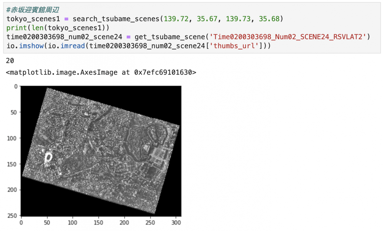
There are 20 scenes taken around the Guest House in Akasaka. You can see the Imperial Palace and Tokyo’s National Stadium in the thumbnails.
# 小石川周辺
# 範囲を指定してシーン情報を取得し個数を表示
tokyo_scenes2 = search_tsubame_scenes(139.74, 35.72, 139.75, 35.73)
print(len(tokyo_scenes2))

# 代表的なシーンのサムネイルを表示
time0200044317_num02_scene62 = get_tsubame_scene('Time0200044317_Num02_SCENE62_RSVLAT1')
io.imshow(io.imread(time0200044317_num02_scene62['thumbs_url']))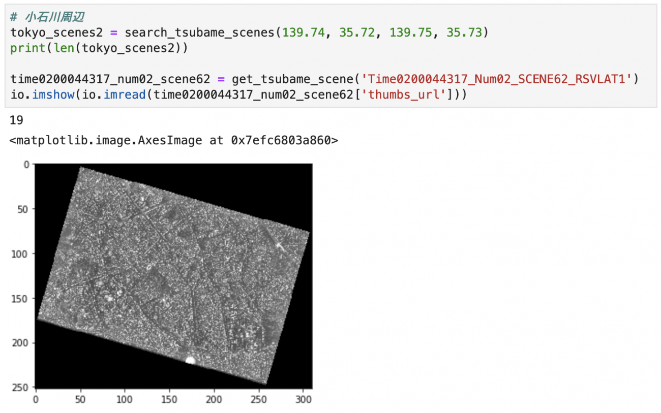
There are 19 scenes taken around Koishikawa. The white semicircle at the bottom of the picture is a part of the Tokyo Dome.
Now, in the same way, we are going to obtain scenes taken in the other three spots.
# ワイキキ
# 範囲を指定してシーン情報を取得し個数を表示
waikiki_scenes = search_tsubame_scenes(-157.8561, 21.2579, -157.7961, 21.3179)
print(len(waikiki_scenes))

# 代表的なシーンのサムネイルを表示
time0198385582_num01_scene38 = get_tsubame_scene('Time0198385582_Num01_SCENE38_RSVLAT1')
io.imshow(io.imread(time0198385582_num01_scene38['thumbs_url']))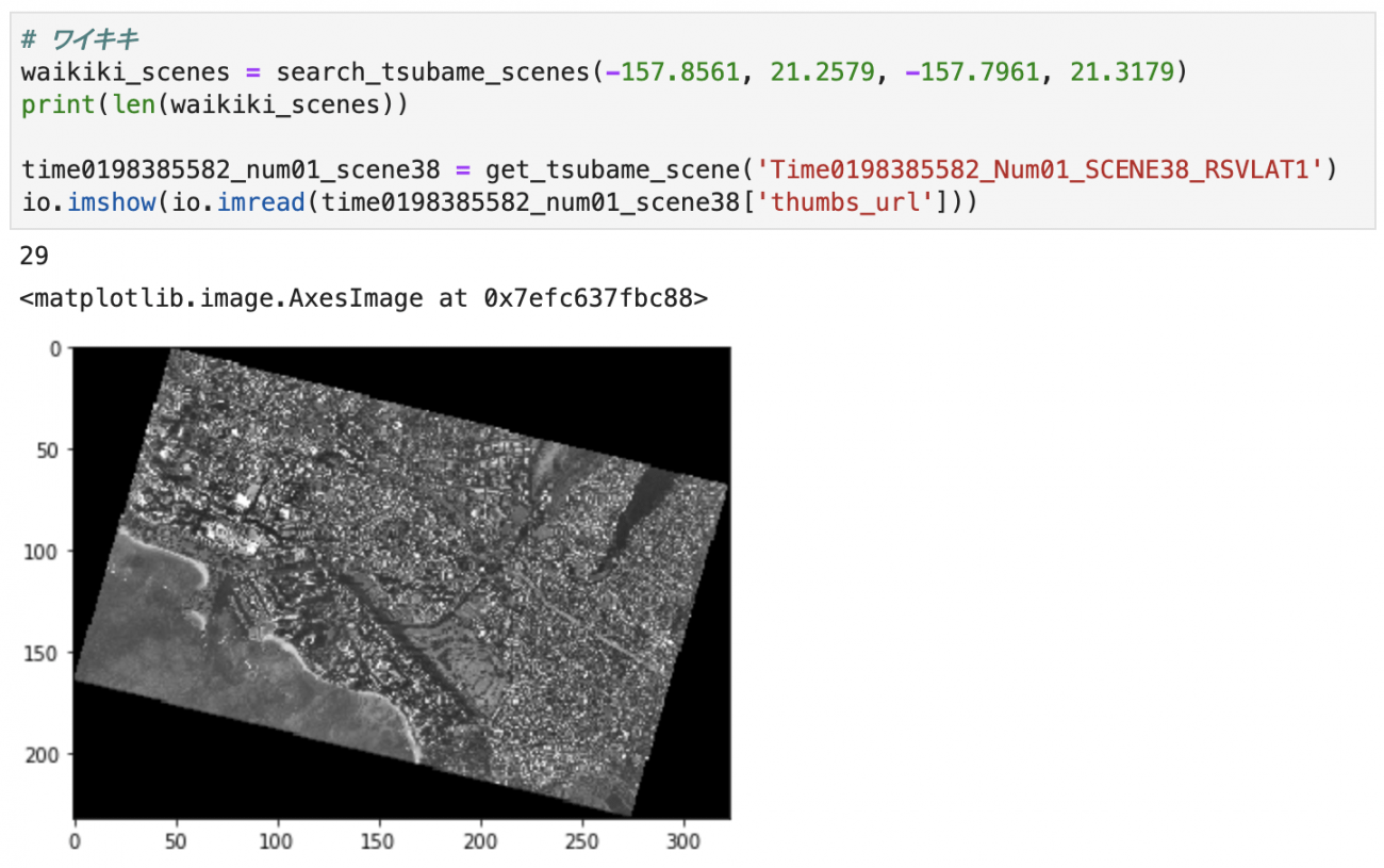
# クウェート 港湾部
# 範囲を指定してシーン情報を取得し個数を表示
kuwait_scenes1 = search_tsubame_scenes(47.9, 29.293, 47.93, 29.323)
print(len(kuwait_scenes1))

# 代表的なシーンのサムネイルを表示
time0196866935_num02_scene28 = get_tsubame_scene('Time0196866935_Num02_SCENE28_RSVLAT1')
io.imshow(io.imread(time0196866935_num02_scene28['thumbs_url']))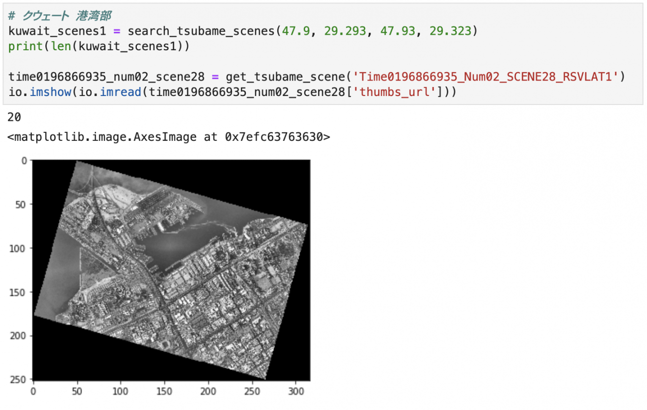
# クウェート 市街地
# 範囲を指定してシーン情報を取得し個数を表示
kuwait_scenes2 = search_tsubame_scenes(47.91, 29.333, 47.94, 29.363)
print(len(kuwait_scenes2))

# 代表的なシーンのサムネイルを表示
time0196866935_num02_scene29 = get_tsubame_scene('Time0196866935_Num02_SCENE29_RSVLAT2')
io.imshow(io.imread(time0196866935_num02_scene29['thumbs_url']))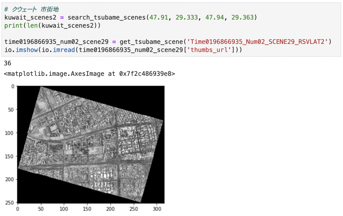
# ニース コートダジュール空港
# 範囲を指定してシーン情報を取得し個数を表示
nice_scenes1 = search_tsubame_scenes(7.197, 43.645, 7.227, 43.675)
print(len(nice_scenes1))

# 代表的なシーンのサムネイルを表示
time0197050489_num02_scene41 = get_tsubame_scene('Time0197050489_Num02_SCENE41_RSVLAT2')
io.imshow(io.imread(time0197050489_num02_scene41['thumbs_url']))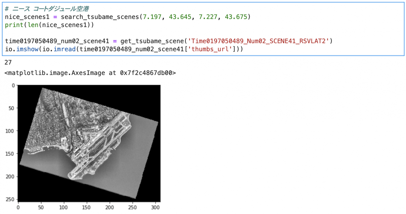
# ニース プロムナード・デ・ザングレ
# 範囲を指定してシーン情報を取得し個数を表示
nice_scenes2 = search_tsubame_scenes(7.211, 43.685, 7.241, 43.715)
print(len(nice_scenes2))

# 代表的なシーンのサムネイルを表示
time0197396345_num04_scene03 = get_tsubame_scene('Time0197396345_Num04_SCENE03_RSVLAT1')
io.imshow(io.imread(time0197396345_num04_scene03['thumbs_url']))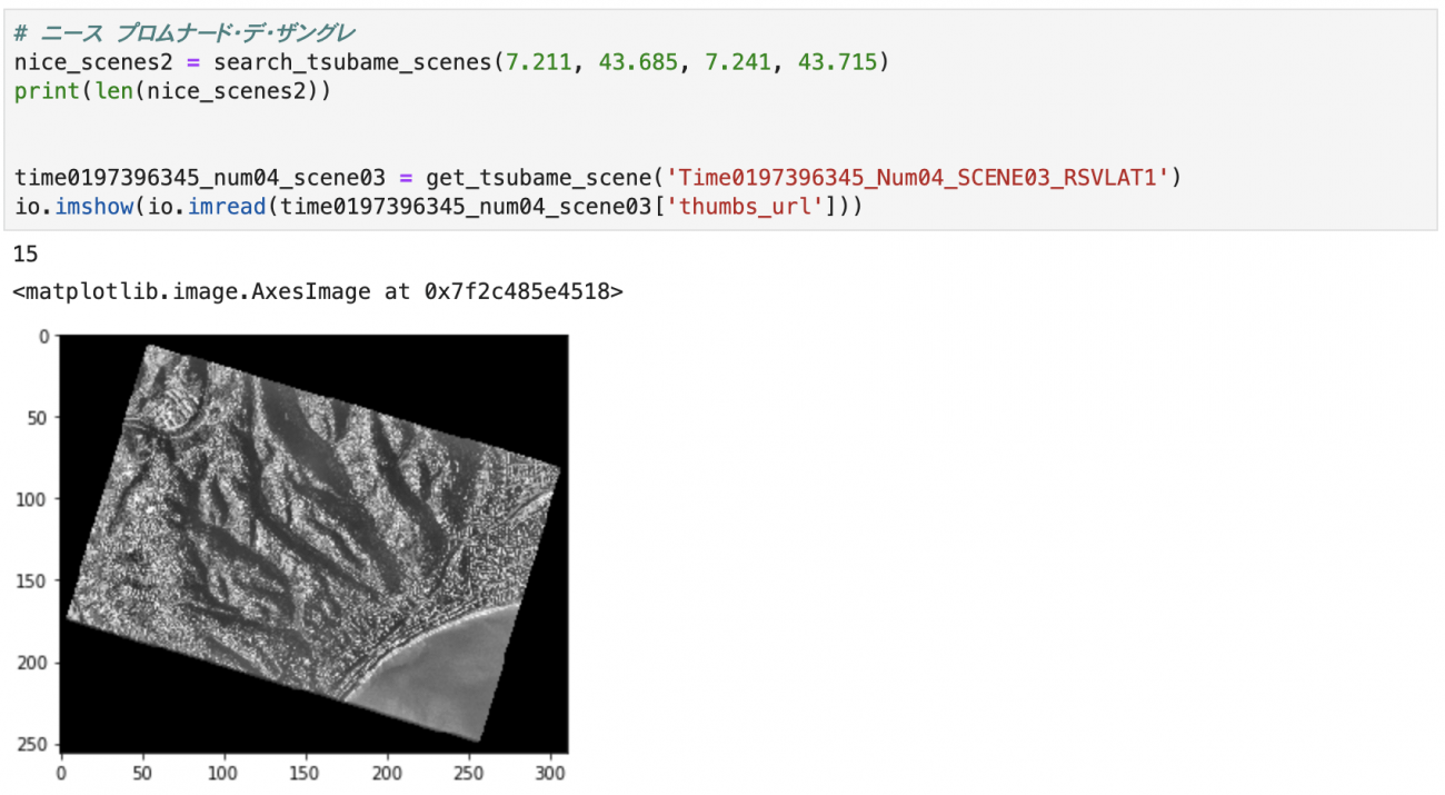
Making animation to observe changes
SLATS periodically carried out observations at almost the same spots in the above four locations.
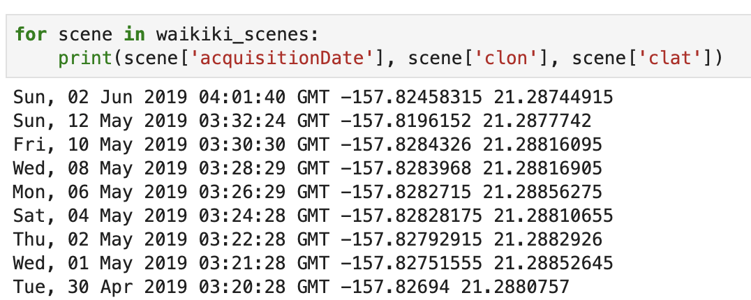
We are taking this opportunity to make animations using these scenes. In this sample code, an animated GIF is created from the thumbnails included in the scene information.
import matplotlib.pyplot as plt
import matplotlib.animation as animation
import dateutil.parser
sorted_scenes = sorted(waikiki_scenes, key=lambda scene: dateutil.parser.parse(scene['acquisitionDate']))

plt.gray()
fig = plt.figure()
ims = []
for s in sorted_scenes:
    ims.append([plt.imshow(io.imread(s['thumbs_url']))])

ani = animation.ArtistAnimation(fig, ims, interval=1000, repeat_delay=1000)
ani.save('tsubame_scenes.gif', writer='pillow')
plt.close()
from IPython.display import HTML
HTML('<img src="tsubame_scenes.gif">')
World landmark observations by SLATS
Here are some scenes taken by SLATS besides the above four locations.
# エジプト ギザ
scene = get_tsubame_scene('Time0201367447_Num02_SCENE42_RSVLAT1')

io.imshow(io.imread(scene['thumbs_url']))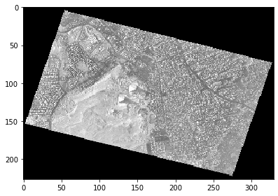
This scene is taken over Giza, Egypt, on May 20, 2019. You can see the two pyramids and the Sphinx in the middle of the image.
# ドバイ The world
scene = get_tsubame_scene('Time0201879426_Num02_SCENE21_RSVLAT1')

io.imshow(io.imread(scene['thumbs_url']))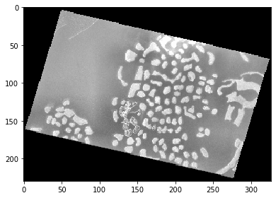
This scene is taken over Dubai on May 26, 2019. You can see the artificial shape of the archipelago called “The World.”
# 北京 紫禁城
scene = get_tsubame_scene('Time0203508565_Num03_SCENE35_RSVLAT1')

io.imshow(io.imread(scene['thumbs_url']))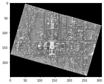
This scene is taken over Beijing on July 14, 2019. You can clearly see the Forbidden City and Tiananmen Square in the middle of the image and the artificial pond, Zhongnanhai, on the left.
# ニューヨーク ペンシルベニア駅
scene = get_tsubame_scene('Time0204678387_Num04_SCENE09_RSVLAT1')

io.imshow(io.imread(scene['thumbs_url']))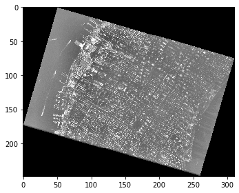
This scene is taken over New York City on July 27, 2019. You can see skyscrapers lined up in the grid patterns of New York City. The round structure in the middle of the screen is Pennsylvania Station.
How do orbit altitude, shooting range, and ground resolution relate to each other?
The relationship among orbit altitude, shooting range, and ground resolution is described below.
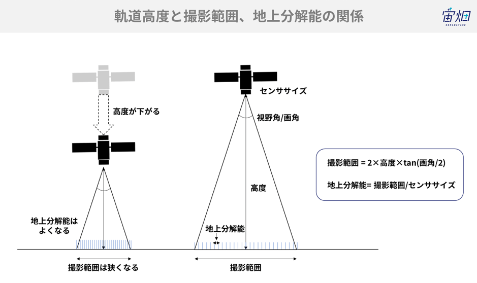
Since the satellite’s sensor size and view angle remain the same, as altitude decreases, the shooting range gets narrower and the ground resolution gets better.
In the case of SLATS, as the orbit altitude was gradually decreasing, more recent images were taken at lower altitude and have a better ground resolution.
In addition, it would be interesting to calculate the shooting range and the ground resolution of a specific date as the view angle of the mounted camera is reported to be 9.1 mrad (observation width of 2 km at 220 kilometers altitude).
We hope now you understand the decommission of a satellite and how to interpret SLATS’ observation data.
There have been plans to develop a successor to SLATS and to operate multiple satellites at the same time. Attention must be paid as to how the achievements of this technical demonstration will be utilized in the future.