We recently introduced various methods of super-resolution in an article titled What you can do with super-resolution and satellite images: an introduction to related papers and how to do it with Tellus. In this article, we will try to perform a method of super-resolution on actual satellite data using Tellus.

Super-resolution is a technique to convert low-resolution images (blurred images) to pseudo-high-resolution images (clearly visible).

Since it is particularly difficult to obtain satellite images of high resolution, this kind of super-resolution technology is very useful. In addition to making it easier for us to recognize what is in a satellite image, super-resolution is also expected to improve the accuracy of object detection for machine learning.

Reference: The Effects of Super-Resolution on Object Detection Performance in Satellite Imagery

There are various methods of super-resolution, but in this article, we will use a basic method of single image super-resolution called SRCNN. For implementation, we use Keras, a machine learning library.

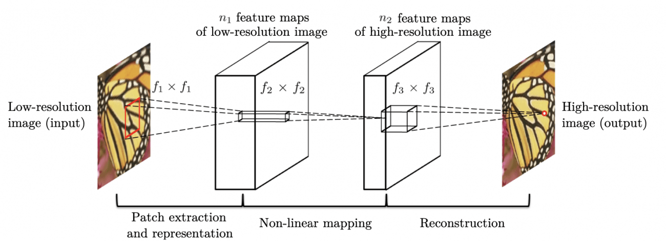
1. Overview of SRCNN (Super-Resolution Convolutional Neural Network)

SRCNN is a method presented in 2014 by Chao Dong et al. The paper is available here. SRCNN, as the name suggests, is a technique that uses CNN for super-resolution. Until then, CNN had not been used for super-resolution, so this was seen as a very innovative method.

SRCNN takes a low-resolution image as input and converts (maps) it to a high-resolution image. It learns this mapping method by using training data.

The great thing about SRCNN is that it is so simple. It has only three layers including the output layer. The first layer corresponds to the extraction of patches, the second layer, to non-linear mapping, and the third layer, to reconstruction (see below).

2. Obtain satellite data

Now let’s get started by super-resolution using the Tellus development environment.

We use the satellite data from ASNARO-1. For more information on how to obtain ASNARO-1 data with Tellus API, please see this article.

The following operations are basically carried out on the development environment of Tellus (JupyterLab). See Tellusの開発環境でAPI引っ張ってみた (Use Tellus API from the development environment) for how to use JupyterLab.

First, create the directory “Data_ASNARO1_SRCNN,” and then run the following code:

import os, json, requests, math
from skimage import io
from io import BytesIO
import matplotlib.pyplot as plt
import warnings
import random
import numpy as np

%matplotlib inline

random.seed(0)

TOKEN = "(トークンを貼り付ける)"

def get_ASNARO_scene(min_lat, min_lon, max_lat, max_lon):
    url = "https://gisapi.tellusxdp.com/api/v1/asnaro1/scene" 
        + "?min_lat={}&min_lon={}&max_lat={}&max_lon={}".format(min_lat, min_lon, max_lat, max_lon)
    
    headers = {
        "content-type": "application/json",
        "Authorization": "Bearer " + TOKEN
    }
    
    r = requests.get(url, headers=headers)
    return r.json()

def get_tile_num(lat_deg, lon_deg, zoom):
    #ズーム率と点(緯度、経度)を与えたときに点を含むタイル座標を求める
    lat_rad = math.radians(lat_deg)
    n = 2.0 ** zoom
    xtile = int((lon_deg + 180.0) / 360.0 * n)
    ytile = int((1.0 - math.log(math.tan(lat_rad) + (1 / math.cos(lat_rad))) / math.pi) / 2.0 * n)
    return (xtile, ytile)

def get_tile_bbox(z, x, y):
    #タイル座標（z, x, y）に対して、その画像の左下と右上の緯度経度を返す。
   
    def num2deg(xtile, ytile, zoom):       #https://wiki.openstreetmap.org/wiki/Slippy_map_tilenames#Python
        n = 2.0 ** zoom
        lon_deg = xtile / n * 360.0 - 180.0
        lat_rad = math.atan(math.sinh(math.pi * (1 - 2 * ytile / n)))
        lat_deg = math.degrees(lat_rad)
        return (lon_deg, lat_deg)
    
    right_top = num2deg(x + 1, y, z)
    left_bottom = num2deg(x, y + 1, z)
    return (left_bottom[0], left_bottom[1], right_top[0], right_top[1])

def get_ASNARO_image(scene_id, zoom, xtile, ytile):
    url = " https://gisapi.tellusxdp.com/ASNARO-1/{}/{}/{}/{}.png".format(scene_id, zoom, xtile, ytile)
    headers = {
        "Authorization": "Bearer " + TOKEN
    }
    
    r = requests.get(url, headers=headers)
    return io.imread(BytesIO(r.content))


# 関東近辺のシーンを取得する。
scene = get_ASNARO_scene(35.2, 138.0, 37.1, 140.5)

# 得られたシーン群の中からランダムに30つ選ぶ。
random_scenes = random.sample(scene, 30)

# ズーム率17で各シーンから切り出せるタイル画像を最大300枚まで取得する。
zoom = 17

for scene in random_scenes:
    count = 0
    
    (xtile, ytile) = get_tile_num(scene['max_lat'], scene['min_lon'], zoom)

    x_len = 0
    while(True):
        bbox = get_tile_bbox(zoom, xtile + x_len + 1, ytile)
        tile_lon = bbox[0]
        if(tile_lon > scene['max_lon']):
            break
        x_len += 1

    y_len = 0
    while(True):
        bbox = get_tile_bbox(zoom, xtile, ytile + y_len + 1)
        tile_lat = bbox[3]
        if(tile_lat < scene['min_lat']):
            break
        y_len += 1

    for x in range(x_len):
        for y in range(y_len):    
            try:
                img = get_ASNARO_image(scene['entityId'], zoom, xtile + x, ytile + y)
                if(np.count_nonzero(np.ravel(img))/len(np.ravel(img)) > 0.99):
                    with warnings.catch_warnings():
                        warnings.simplefilter('ignore')                   
                        io.imsave(os.getcwd()+
'/Data_ASNARO1_SRCNN/{}_{}_{}.png'.format(zoom,
 xtile + x, ytile + y), img)
                        count += 1
            except Exception as e:
                print(e)
            #取得枚数が300枚を超えたら次のシーンへ移る。
            if count >= 300:
                break
        else:
            continue
        break

It’s going to take a fair amount of time, so please be patient (about 30 minutes in our case).

After waiting, we got 6,616 images. Randomly divide these into 6,000 train images and 616 test images. The data structure is as follows:
●Data Structure

┗  Data_ASNARO1_SRCNN
┣ train (6000)
┗ test (616)

3. Load the data and define the model

Now that we have the data ready, let’s implement SRCNN using Keras. First, install the necessary libraries.

from keras import backend as K
from keras.models import Sequential, Model, load_model
from keras.layers import Input, Dense, Input, Conv2D, Conv2DTranspose, MaxPooling2D, UpSampling2D, Lambda, Activation, Flatten, Add
from keras.optimizers import Adam, SGD
from keras.preprocessing.image import array_to_img, img_to_array, load_img,ImageDataGenerator

For training, we need a pair of high-resolution images (correct data) and low-resolution images (input data). However, the size of the input and output images are the same in the SRCNN network. For this reason, we need to use rough images as input data, which can be generated by enlarging low-resolution images to the same size as high-resolution images in the classical manner.
For this purpose, we first reduce the size of the ASNARO-1 high-resolution image (correct answer) by four times and enlarge it again to the original size, which is then used as input data.

So let’s load the data.

def drop_resolution(x,scale):
   #画像のサイズをいったん縮小したのちに再び拡大することで、低解像度の画像を作る。
   size=(x.shape[0],x.shape[1])
   small_size=(int(size[0]/scale),int(size[1]/scale))
   img=array_to_img(x)
   small_img=img.resize(small_size, 3)
   return img_to_array(small_img.resize(img.size,3))

def data_generator(data_dir,mode,scale,target_size=(256,256),batch_size=32,shuffle=True):
   for imgs in ImageDataGenerator().flow_from_directory(
       directory=data_dir,
       classes=[mode],
       class_mode=None,
       color_mode='rgb',
       target_size=target_size,
       batch_size=batch_size,
       shuffle=shuffle
   ):
       x=np.array([
           drop_resolution(img,scale) for img in imgs
           ])
       yield x/255.,imgs/255.


DATA_DIR='./Data_ASNARO1_SRCNN/'
N_TRAIN_DATA=6000　#学習用データ数
N_TEST_DATA=616　　#評価用データ数
BATCH_SIZE=32　　　#バッチサイズ

train_data_generator=data_generator(
   DATA_DIR,'train', scale=4.0, batch_size=BATCH_SIZE
)

test_x,test_y=next(
   data_generator(
   DATA_DIR,'test',scale=4.0, batch_size=N_TEST_DATA,shuffle=False
   )
)

The next step is to define the network configuration for SRCNN. This time, we adapt the parameter values that are used as criteria in the original paper. That is, the number of filters (64, 32, 3) and the kernel size (9,1,5) are applied to the first, second and third layers, respectively.

model = Sequential()

model.add(Conv2D(filters=64, kernel_size= 9, activation='relu', padding='same', input_shape=(None,None,3)))
model.add(Conv2D(filters=32, kernel_size= 1, activation='relu', padding='same'))
model.add(Conv2D(filters=3, kernel_size= 5, padding='same'))

model.summary()

The great thing about Keras is that we can configure a network with just a few lines.

4. Train models

Now, it is time to train models. But before that, note that the PSNR (Peak Signal to Noise Ratio) is commonly used as the evaluation function in the field of super-resolution.

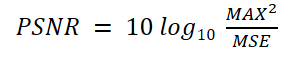
MAX is the maximum value that the correct data can take, which in this case is 1.0, and MSE is the mean square error between the output result and the correct data. Since the MSE is the denominator, the closer the output is to the correct data, the smaller the MSE and the larger the PSNR. The unit is in dB (decibels).

So we first define this PSNR as a function.

def psnr(y_true,y_pred):
    return -10*K.log(K.mean(K.flatten((y_true-y_pred))**2)
    )/np.log(10)

Then, we compile the model and use the training data to train the network.

For the loss function, we used MSE (mean square error) according to the original paper and Adam as an optimizer. In this case, it learns 200 epochs.

model.compile(
    loss='mean_squared_error',
    optimizer= 'adam',
    metrics=[psnr]
)

model.fit_generator(
    train_data_generator,
    validation_data=(test_x,test_y),
    steps_per_epoch=N_TRAIN_DATA//BATCH_SIZE,
    epochs=200
)

When the learning process begins, the following output is produced: It takes a considerable amount of time (about a couple of days). If you want to make this calculation even faster, you might want to sign up for Tellus’ GPU plan.

Epoch 1/200
Found 6000 images belonging to 1 classes.
187/187 [==============================] - 50s 270ms/step - loss: 0.0124 - psnr: 19.4878 - val_loss: 0.0094 - val_psnr: 20.7444
Epoch 2/200
187/187 [==============================] - 47s 253ms/step - loss: 0.0094 - psnr: 20.3751 - val_loss: 0.0084 - val_psnr: 21.2547
Epoch 3/200
187/187 [==============================] - 47s 253ms/step - loss: 0.0086 - psnr: 20.7265 - val_loss: 0.0076 - val_psnr: 21.6969
Epoch 4/200
187/187 [==============================] - 47s 253ms/step - loss: 0.0078 - psnr: 21.1911 - val_loss: 0.0072 - val_psnr: 22.0746
Epoch 5/200
187/187 [==============================] - 47s 251ms/step - loss: 0.0081 - psnr: 21.0456 - val_loss: 0.0114 - val_psnr: 20.6750
.
.
.
.
.
Epoch 195/200
187/187 [==============================] - 47s 250ms/step - loss: 0.0049 - psnr: 23.2101 - val_loss: 0.0049 - val_psnr: 23.7697
Epoch 196/200
187/187 [==============================] - 47s 251ms/step - loss: 0.0050 - psnr: 23.1422 - val_loss: 0.0053 - val_psnr: 23.2070
Epoch 197/200
187/187 [==============================] - 47s 251ms/step - loss: 0.0049 - psnr: 23.1455 - val_loss: 0.0049 - val_psnr: 23.7604
Epoch 198/200
187/187 [==============================] - 47s 250ms/step - loss: 0.0049 - psnr: 23.2479 - val_loss: 0.0053 - val_psnr: 23.3400
Epoch 199/200
187/187 [==============================] - 47s 252ms/step - loss: 0.0050 - psnr: 23.0964 - val_loss: 0.0051 - val_psnr: 23.5275
Epoch 200/200
187/187 [==============================] - 47s 249ms/step - loss: 0.0050 - psnr: 23.1375 - val_loss: 0.0049 - val_psnr: 23.8679

Well, now the learning is done. The PSNR values in the final epoch are 23.14. for the training data and 23.87. for the test data.

5. Generate high-resolution images with trained models

Finally, it’s time to use the trained model to construct a high-resolution image. Provide a test image degraded to a lower resolution as input and convert it to a higher resolution image.

pred=model.predict(test_x)

Now we have a high-resolution image as predicted by SRCNN. Let’s look at the converted high-resolution images. We will look at one test image to see how it works.

fig = plt.figure(figsize=(50,50), facecolor="w")
N_show = 229 #N_show番目の評価用データを表示。

plt.subplot(1,3,1)
plt.title("Orignial",fontsize=80)
plt.tight_layout()
plt.imshow(test_y[N_show,:,:])

plt.subplot(1,3,2)
plt.title("Low resolution",fontsize=80) 
plt.tight_layout()
plt.imshow(test_x[N_show,:,:])

plt.subplot(1,3,3)
plt.title("SRCNN result",fontsize=80)
plt.tight_layout()
plt.imshow(pred[N_show,:,:])

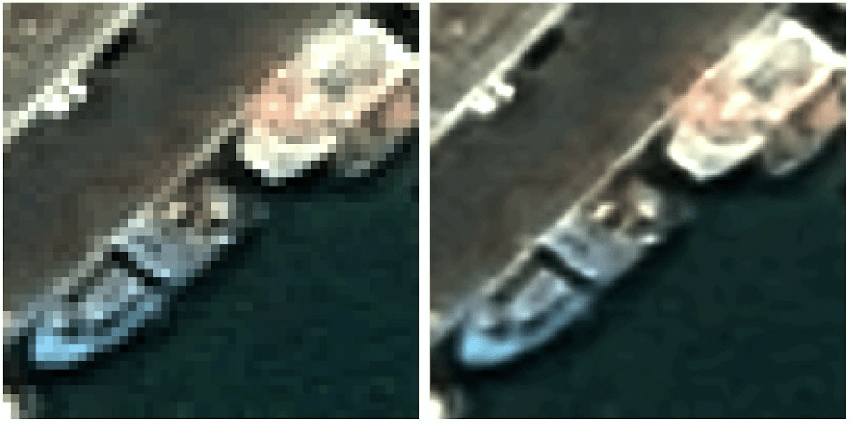
Then the following images of the city were displayed. The left side is the original high-resolution image, the middle is the low-resolution image given as input, and the right side is the high-resolution image converted by SRCNN.

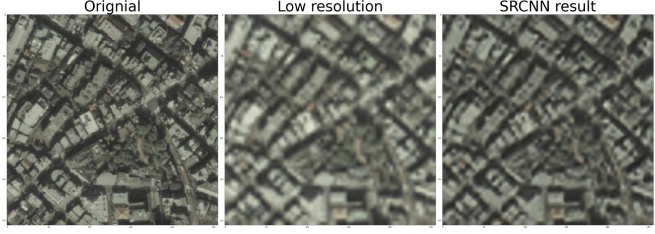
The SRCNN image has a clearer outline of the building than the input image. The PSNR value for this image, constructed by SRCNN, was 25.78.

Let’s also look at another place. Now here are images of a rural area.

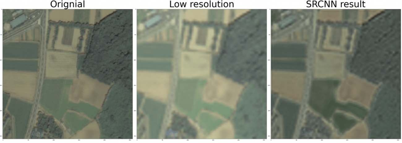
The outline of the rice fields and forests became clearer here too, thanks to the high-resolution imaging of the SRCNN. The PSNR value for this image, constructed by SRCNN, was 28.73.

As other studies (e.g., this article) have shown, super-resolution in urban areas is less accurate than in rural areas.

6. Summary

This time, we performed super-resolution using SRCNN for a satellite image of ASNARO-1 downloaded using Tellus.

As shown in the original paper proposing SRCNN, the performance of the SRCNN’s model also varies with the number of filters, kernel size, number of layers, etc. We have configured the network with the standard parameter settings, but you may want to experiment with some of these parameters to see if you can get more super-resolution accuracy.

Also, as mentioned in the previous article, “What you can do with super-resolution and satellite images: an introduction to related papers and how to do it with Tellus,” super-resolution has been actively studied in recent years, and various other methods have emerged, including the use of GANs. If you’re interested, please read this article and the original paper and try to apply it to satellite data (and, of course, other data).

* Reference articles and books that were not cited in the article

-“An Introduction to TensorFlow Development: Building Deep Learning Models with Keras” by Mitsuhisa Ohta, Kodai Sudo, Takuma Kurosawa, and Daisuke Oda

–“Deep-Learning-Based Super Resolution for Satellite Imagery” (2018) by Issei Kawashima and Ryosuke Nakamura

Try using satellite data on “Tellus”!

Want to try using satellite data? Try out Japan’s open and free to use data platform, “Tellus”!
You can register for Tellus right here