AI (Artificial Intelligence) has now become pretty common in much of the business world.
In the satellite data field, applications of AI such as machine learning and deep learning are capturing more and more attention every year.

Given the situation, we, the Sorabatake editorial department, could say, “AI looks too difficult for us…” no more.
We have to study AI right now to prepare for the coming age of AI, or we will be left behind in the industry…

The important thing is always to give it a try.

In this article, you will see how we have tried to use AI for satellite data handling (and also how we struggled!).

*This article is part 16 of the “Space Data Utilization” series in which SORABATAKE members introduce interesting people and things related to satellite images. Your views and advice are welcome and will be gladly heard at any time.

1) Decide what to do using AI

First, think about what to do using AI. Detection of cars and buildings, estimation of threshold values, noise removal, etc.

There are many things we want AI to do to make use of satellite data. However, if beginners start with difficult things, perhaps they won’t be able to handle them and will then give up.

After some consideration, we decided to do a simple binary classification to determine whether images have clouds in them or not.

Optical satellite imagery often doesn’t let you see your target points on the ground because of clouds, even though you can find images of your target areas. That’s how optical observation works.

Clouds make it hard to compare images of the same point captured at different times, so it would be useful for analytical purposes if you could group images according to whether they have clouds or not. We gave it a spin, with little idea how easy or hard it was.

2) Get tiles of AVNIR-2 imagery

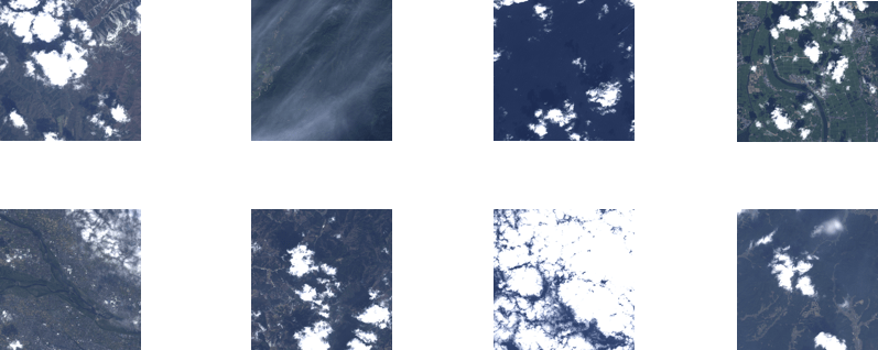
First, get satellite images to classify. Here, we use optical satellite data from AVNIR-2.

Select about 30 random scenes from AVNIR-2 imagery. Then, cut tiles out of the scenes at a zoom factor of 12 and save them.

All the following operations are carried out on the development environment of Tellus (JupyterLab) development environment.
See Tellusの開発環境でAPI引っ張ってみた (Use Tellus API from the development environment) for how to use JupyterLab.

import os
import requests
import math
from skimage import io
from io import BytesIO
import random
import warnings
import numpy as np


TOKEN = 'アクセストークンを貼ってください。'
DOMAIN = 'tellusxdp.com'

def search_AVNIR2_scenes(min_lon, min_lat, max_lon, max_lat):
    url = 'https://gisapi.{}/api/v1/av2ori/scene'.format(DOMAIN)
    headers = {
        'Authorization': 'Bearer ' + TOKEN
    }
    payload = {'min_lat': min_lat, 'min_lon': min_lon,
               'max_lat': max_lat, 'max_lon': max_lon}

    r = requests.get(url, params=payload, headers=headers)
    if r.status_code is not 200:
        raise ValueError('status error({}).'.format(r.status_code))
    return r.json()

def get_AVNIR2_scene_tile(rsp_id, product_id, zoom, xtile, ytile,
                            opacity=1, r=3, g=2, b=1, rdepth=1, gdepth=1, bdepth=1, preset=None):
    # zoom = 8 - 14
    url = 'https://gisapi.{}/av2ori/{}/{}/{}/{}/{}.png'.format(
        DOMAIN, rsp_id, product_id, zoom, xtile, ytile)
    headers = {
        'Authorization': 'Bearer ' + TOKEN
    }

    payload = {'preset': preset, 'opacity': opacity, 'r': r, 'g': g,
               'b': b, 'rdepth': rdepth, 'gdepth': gdepth, 'bdepth': bdepth}

    r = requests.get(url, params=payload, headers=headers)
    if not r.status_code == requests.codes.ok:
        r.raise_for_status()
    return io.imread(BytesIO(r.content))

def get_tile_num(lat, lon, zoom):
    """
    緯度経度からタイル座標を取得する
    """
    # https://wiki.openstreetmap.org/wiki/Slippy_map_tilenames#Python
    lat_rad = math.radians(lat)
    n = 2.0 ** zoom
    xtile = int((lon + 180.0) / 360.0 * n)
    ytile = int((1.0 - math.log(math.tan(lat_rad) + (1 / math.cos(lat_rad))) / math.pi) / 2.0 * n)
    return (xtile, ytile)

def get_tile_bbox(z, x, y):
    """
    タイル座標からバウンディングボックスを取得する
    https://tools.ietf.org/html/rfc7946#section-5
    """
    def num2deg(xtile, ytile, zoom):
        # https://wiki.openstreetmap.org/wiki/Slippy_map_tilenames#Python
        n = 2.0 ** zoom
        lon_deg = xtile / n * 360.0 - 180.0
        lat_rad = math.atan(math.sinh(math.pi * (1 - 2 * ytile / n)))
        lat_deg = math.degrees(lat_rad)
        return (lon_deg, lat_deg)
    
    right_top = num2deg(x + 1, y, z)
    left_bottom = num2deg(x, y + 1, z)
    return (left_bottom[0], left_bottom[1], right_top[0], right_top[1])

# 日本周辺のシーン情報を取得し、ランダムに30シーン絞り込み
scenes = search_AVNIR2_scenes(120.0, 24.0, 155.0, 46.0)
random_scenes = random.sample(scenes, 30)


# ズーム率12でそのシーンから切り出せるタイル画像をすべて取得する
zoom = 12
for scene in random_scenes:
    (xtile, ytile) = get_tile_num(scene['max_lat'], scene['min_lon'], zoom)

    x_len = 0
    while(True):
        bbox = get_tile_bbox(zoom, xtile + x_len + 1, ytile)
        tile_lon = bbox[0]
        if(tile_lon > scene['max_lon']):
            break
        x_len += 1

    y_len = 0
    while(True):
        bbox = get_tile_bbox(zoom, xtile, ytile + y_len + 1)
        tile_lat = bbox[3]
        if(tile_lat < scene['min_lat']):
            break
        y_len += 1

    for x in range(x_len):
        for y in range(y_len):    
            try:
                img = get_AVNIR2_scene_tile(scene['rspId'], scene['productId'], zoom, xtile + x, ytile + y)
                if(np.sum(np.ravel(img))) > 0:
                    with warnings.catch_warnings():
                        warnings.simplefilter('ignore')
                        io.imsave(os.getcwd()+'/tile/{}_{}_{}.png'.format(zoom, xtile + x, ytile + y), img)
            except Exception as e:
                print(e)

Create a directory called “tile” and then run the sample code above.

Wait for several minutes until you get all the tiles.

You will have some 3,000 tiles saved in the directory

3) Prepare teacher data

Now you’ve got the materials, but you still lack something to start machine learning.

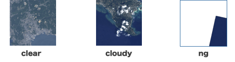
You need teacher data that shows the AI how to distinguish clear and cloudy images.

Create three directories for clear, cloudy and ambiguous images. Then, choose all the clear and cloudy ones from the 3,000 images by looking at each of them with your own eyes.

Who does that daunting task? Humans. I mean if you want to really conduct machine learning properly, you, who are reading this article, need to do this yourself.

In the Sorabatake editorial department, two of us did this task together.
We were grouping images for hours. We hope we will never have to do that again.

We got about 600 clear images and about 1,000 cloudy in our case (unfortunately, the rest were images that were filled with the sea surface or cut off inappropriately).
Both clear and cloudy images are further grouped into “train”, “validation” and “test”. We determined the number of images for each group by intuition.

Structure of the directories and the numbers of images assigned to them

dataset
┣ train (for training)
┃　┣ clear (200)
┃　┗ cloudy (400)
┃
┣ validation (for the validation process in training)
┃　┣ clear (200)
┃　┗ cloudy (400)
┃
┗ test (for evaluation)
┣ clear (200)
┗ cloudy (200)

4) Create a learning model

You’ve finally got all the necessary images. Now, go on to write the code for the AI.

Here, we use TensorFlow as the machine learning framework and Keras as the specialized front-end library for neural networks because plenty of information about them is available on the Internet (both are pre-installed on the development environment of Tellus).

Keras: The Python Deep Learning library

The algorithm called convolutional neural network (CNN) is one of the most common deep learning methods for image processing amongst many.

Using a CNN, you can handle two-dimensional data without breaking it down to one-dimensional pieces (that is, you can deal with the position information of pixels as is), so it is said to be a specialized algorithm for image processing.

[Reference]

画像処理でよく使われる畳み込みニューラルネットワークとは (provisional English title: What is a convolutional neural network, which is often used for image processing?
Deep Learning for Computer Vision – Introduction to Convolution Neural Networks

You need to determine parameters, such as number of filters and size, before you create a CNN model.

Parameter setting is the key point of CNN. It should give a good engineer the opportunity of showing his skill, but we were mere beginners with no idea.

So we had to consult some documents to set values that seemed acceptable. We modified a famous model called VGG16 to use fewer filters in order to reduce the calculation time.

You may be worried about reduced accuracy due to fewer filters, but let’s see how it works.

from keras import layers
from keras import models
from keras import optimizers
from keras.layers import GlobalAveragePooling2D

# 画像サイズ
input_width = 256
input_height = 256

# 畳み込みニューラルネットワーク
model = models.Sequential()
model.add(layers.Conv2D(64, (3, 3), activation='relu', padding='same', 
                        input_shape=(input_width, input_height, 3)))
model.add(layers.MaxPooling2D((2, 2)))
model.add(layers.Conv2D(128, (3, 3), activation='relu', padding='same'))
model.add(layers.MaxPooling2D((2, 2)))
model.add(layers.Conv2D(256, (3, 3), activation='relu', padding='same'))
model.add(layers.MaxPooling2D((2, 2)))
model.add(GlobalAveragePooling2D())
model.add(layers.Dense(256, activation='relu'))
model.add(layers.Dense(1, activation='sigmoid'))

model.compile(loss='binary_crossentropy', optimizer=optimizers.RMSprop(lr=1e-4), 
              metrics=['acc'])

model.summary()

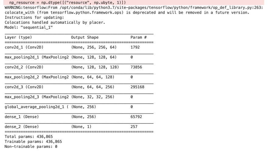
The summary of the model (don’t worry about the WARNING).
The total number of parameters was 436,865.

After creating a model, read the “train” and “validation” data.
Keras’ ImageDataGenerator function creates new images to make up for any shortage of existing ones by randomly rotating, shrinking and enlarging.

It’s a convenient function, but if you fabricate too many images from a limited number of originals in this way, the AI ends up with too many similar ones; so accuracy for the training data would be improved, but it would deteriorate for other data (overtraining).

The batch sizes (a batch size is the number of images used in one iteration) for train and validation data are both set to 30 in this case.

from keras.preprocessing.image import ImageDataGenerator

train_dir = './dataset/train'
validation_dir = './dataset/validation'

# 回転や拡大縮小によりデータ数を水増し
train_datagen = ImageDataGenerator(
    rescale=1./255,
    rotation_range=30,
    width_shift_range=0.1,
    height_shift_range=0.1,
    shear_range=0.1,
    zoom_range=0.1,
    horizontal_flip=True,)

test_datagen = ImageDataGenerator(rescale=1./255)

# 学習用データ読込み
train_generator = train_datagen.flow_from_directory(
        train_dir,
        target_size=(input_width, input_height),
        batch_size=30,
        class_mode='binary')

# 訓練時検証用データ読込み
validation_generator = test_datagen.flow_from_directory(
        validation_dir,
        target_size=(input_width, input_height),
        batch_size=30,
        class_mode='binary')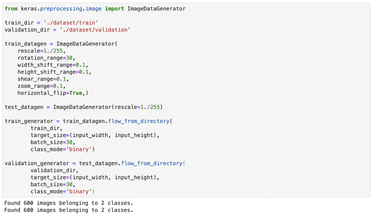

If you get an output other than “Found [the number of the images] images belonging to 2 classes”, there might be unnecessary directories (hidden directories such as. ipynb_checkpoints). You can’t classify your images properly with unnecessary directories. If there are any, remove them and retry.

5) Start training

Finally, set the epoch number (the number of iterations over the entire dataset) and step number, and then start the training.

history = model.fit_generator(
      train_generator,
      steps_per_epoch=100,
      epochs=20,
      validation_data=validation_generator,
      validation_steps=20)

# 処理時間が長いため途中から再開できるようできた学習モデルを保存しておく
model.save('avnir2demo')

In our case, 100 iterations of 100 steps for training and 20 for validation.

Run the code.
And just wait until it’s finished.

Wait.

Wait.

It never ends!

This process kept us waiting for six hours.

We conducted this calculation on the normal development environment of Tellus (4-core CPU & 8GB of RAM).
We hadn’t had any trouble carrying out simple calculations in the environment, but it seemed to be much too slow for deep learning.
We understood why people say you need a GPU for deep learning.

Anyway, let’s check the output.

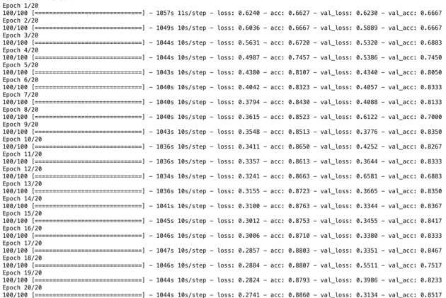
Look at the last line. “val_acc: 0.8517” means it achieved an accuracy of about 85 percent in classifying the validation data after 20 epochs.

You can also see from the records that the accuracy remained much the same after some 10 epochs. Half the number of the iterations might have been enough.

6) Test the model

Test the learning model you’ve created against test data.

from keras.models import load_model
from keras.preprocessing.image import ImageDataGenerator
model = load_model('avnir2demo')     

test_dir = './dataset/test/'
test_datagen = ImageDataGenerator(rescale=1./255)
test_generator = test_datagen.flow_from_directory(
    test_dir,
    target_size=(input_width,input_height),
    batch_size=30,
    class_mode='binary')

test_loss, test_acc = model.evaluate_generator(test_generator, steps=10)
print('test loss:', test_loss)
print('test acc:', test_acc)

In our case, it achieved a very high accuracy of about 88 percent in classifying the test data, too. Fantastic.

But did it really classify the images correctly?
Let’s check the results using some test images one by one.
Below is a sample code for it. Change the file name to match yours.

from skimage import io
import numpy as np
from skimage.transform import resize
%matplotlib inline


img = io.imread('./dataset/test/{clear or cloudy}/{z_x_y}.png')
io.imshow(img)
pred = model.predict(np.expand_dims(img[:,:,0:3]/255, axis=0))
print(pred)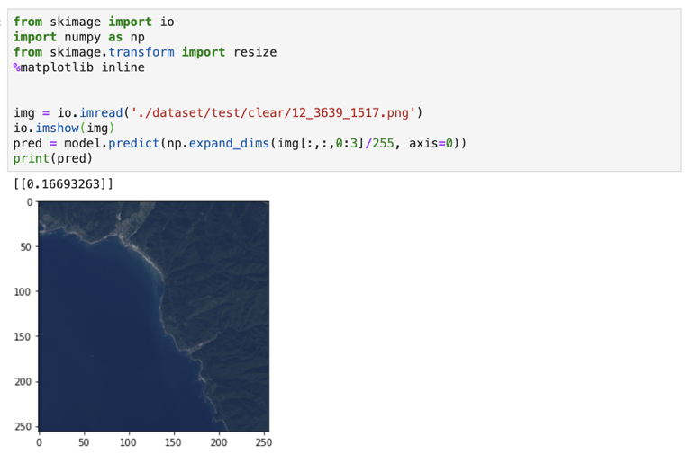

The learning model correctly classified a clear image that had no hint of clouds, returning an expected value (< 0.5).

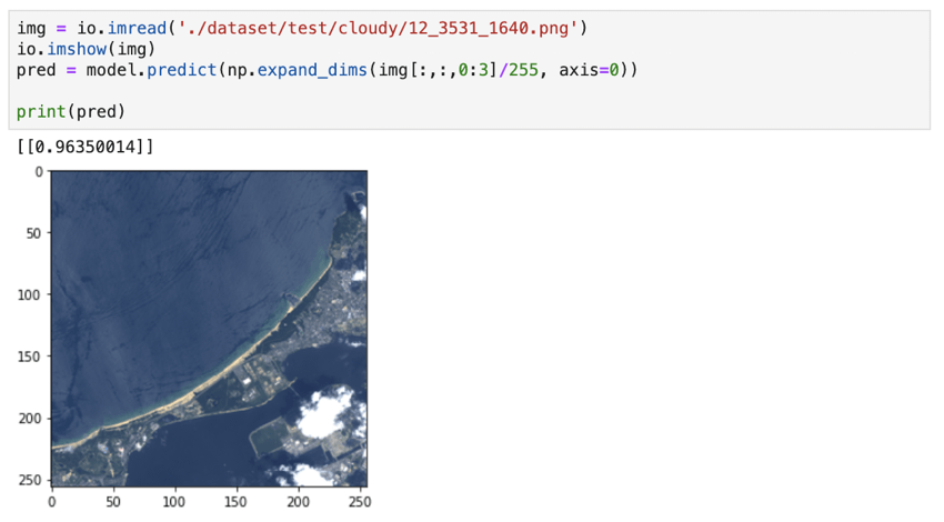
Next, we gave it an image that had some clouds in its bottom right corner. It correctly classified the image as cloudy (≥ 0.5).

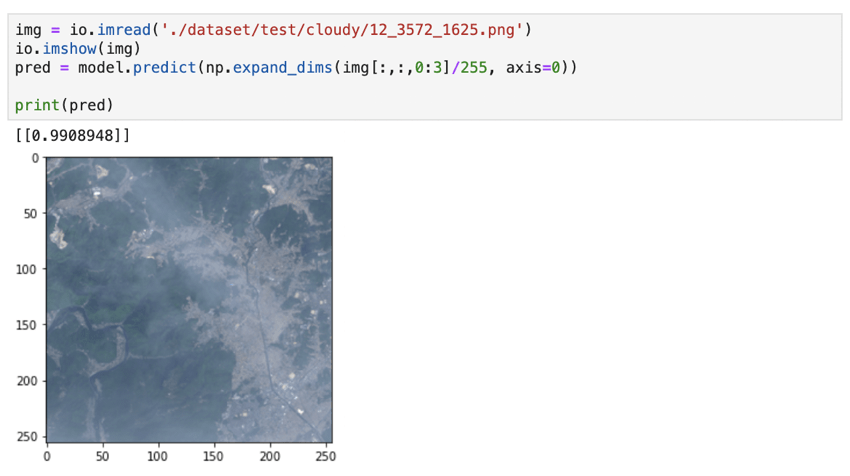
We also presented to it a slightly cloudy image, which was harder to judge. It correctly classified it as cloudy as well.

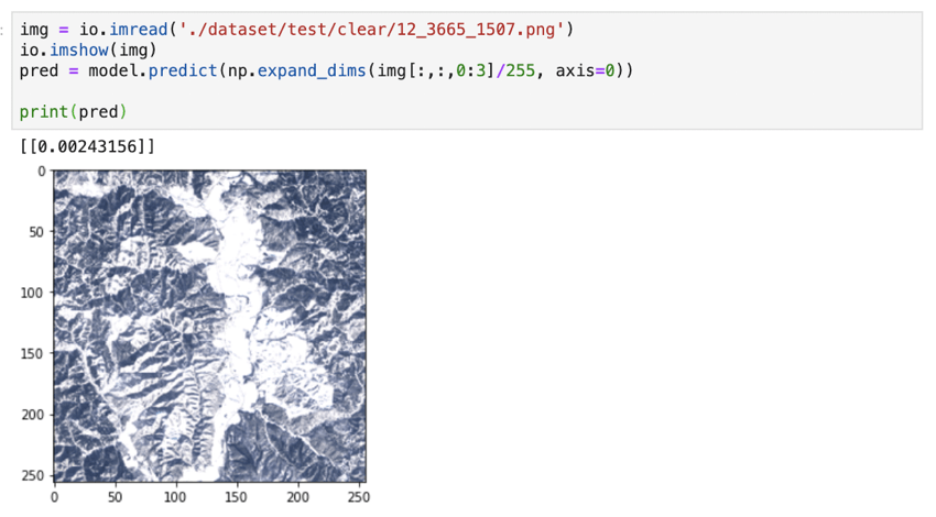
We checked if it was able to correctly classify an image of snow-covered mountains under a clear sky. It managed to give us the correct answer.

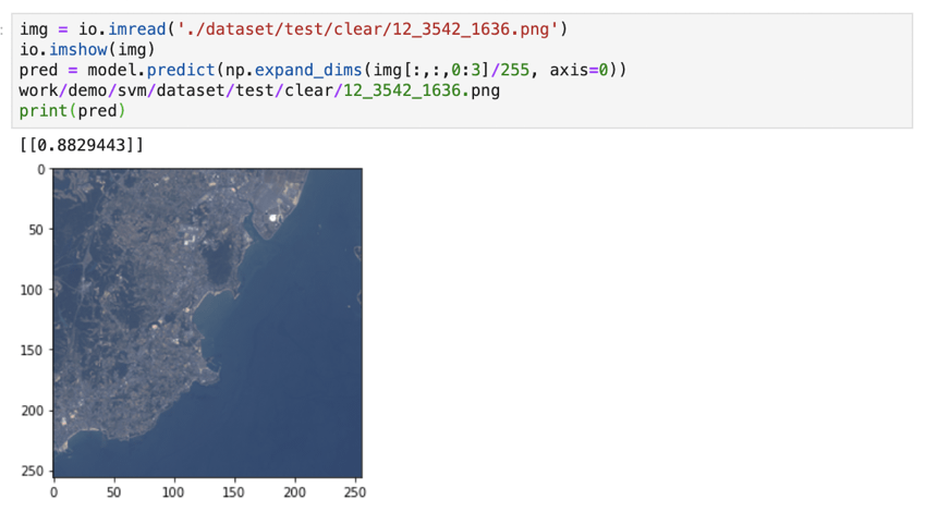
However, it mistook some clear images as cloudy. Maybe it misinterpreted white buildings on the ground as clouds.

7) Summary

As you saw, we were beginners and we just followed an existing example of machine leaning, but we achieved an accuracy of almost 90 percent in judging whether images had clouds or not.

It looks like we could have improved the accuracy by tuning parameters or adding to the teacher data.

After reading this article, do you think you could do something yourself using AI and satellite data?
We’d like you to refer to documents by experts for further study on deep learning, but the Sorabatake editorial department will continue to give you example uses of AI for satellite data, while trying to use AI ourselves.

We also encourage you to try to make use of AI with satellite data and if any easy-to-implement ideas strike you, contributions will be enthusiastically welcomed, so please don’t be shy!