The ALOS-3 is an artificial satellite, planned for launch in 2021. Its main characteristics are, it has an incredibly high ground-level resolution of 0.8 m, and a swath of 70 km, allowing for wide pictures. This means that it can capture photos that cover the entire of Japan as quickly as once a month.

In anticipation of ALOS-3, there is data available on Tellus that resembles the data it will produce, and in this article, we will be showing examples of that data, as well as how you can use its API on the development platform.
*The data is a processed version of World View data (product name: AW3D), which is observed on a technically different wavelength band than with ALOS-3.

Furthermore, the10 images below are the pseudo ALOS-3 data currently available.
①Nagano City: 3 mosaic images taken between 2016/06/03–2019/12/25
②Fukuoka City: 3 mosaic images taken between 2015/04/18–2019/5/15
③Hanoi: 2 mosaic images taken between 2017/12/20–2019/11/25
④Manila: 2 mosaic images taken between 2018/05/12–2019/10/13

*To follow along with the content presented in this article, you’ll need to create an account on Tellus.

(1) View the Pseudo ALOS-3 data on Tellus OS.

The mock ALOS-3 data is available on the Tellus OS library tab under “high-resolution optics | mock ALOS-3 data”.
To view Fukuoka City’s data, enter “Fukuoka Airport” in the search bar and you will get the following results, which show “high-resolution optics | mock ALOS-3 data”.

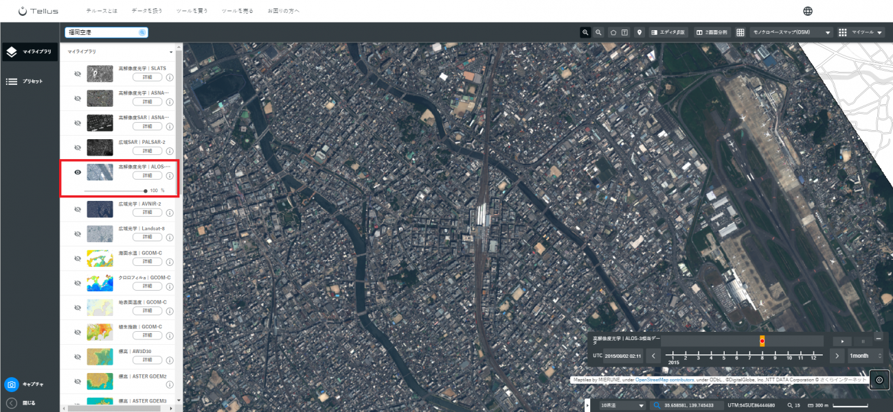
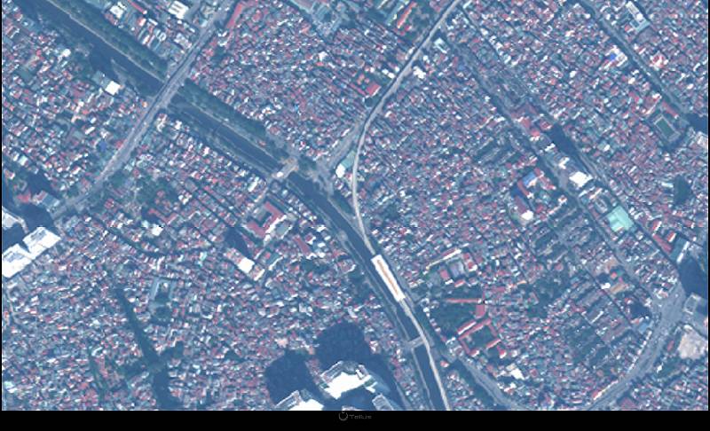
You can clearly see the outlines of houses and also make out the airplanes on the runway in the photo. The following image shows Hanoi, which showcases more complexly shaped houses. You can really feel the difference in culture between the two countries.

This data is also available in 6 different observational wavelength bands. Band 1 is for coastal regions, which allows you to see underwater, and band 5 is for a red edge, which is good for capturing changes in vegetation.

Band 1 0.40–0.45 µm (coastal)
Band2　0.45–0.51 µm (blue)
Band 3 0.52～0.58 µm (green)
Band 4 0.63～0.69 µm (red)
Band 5 0.70–0.74 µm (red edge)
Band 6 0.77–0.89 µm (NIR)

Try the various wavelengths out for yourself on Tellus OS.
Next, we will take a look at how you can view the mock ALOS-3 data on the development environment.

(2) View the Pseudo ALOS-3 Data as an Image on the Development　Environment

The mock ALOS-3 data can be viewed by using the next 4 steps.

1. File Search
Search for the file with metadata that matches your desired requirements.
↓
2. Acquire the Download URL
Create a URL from the file’s metadata to download the file.
↓
3. Download the File
Download the file from the acquired URL into the development environment and click save.

4. Display the Images
Create and display images for each band downloaded from the file.

See “Use Tellus API from the development environment” for information on how to use Jupyter Notebook on Tellus.

File Search API
The following API is used to search for files.

https://file.tellusxdp.com/api/v1/origin/search/alos3-pseudo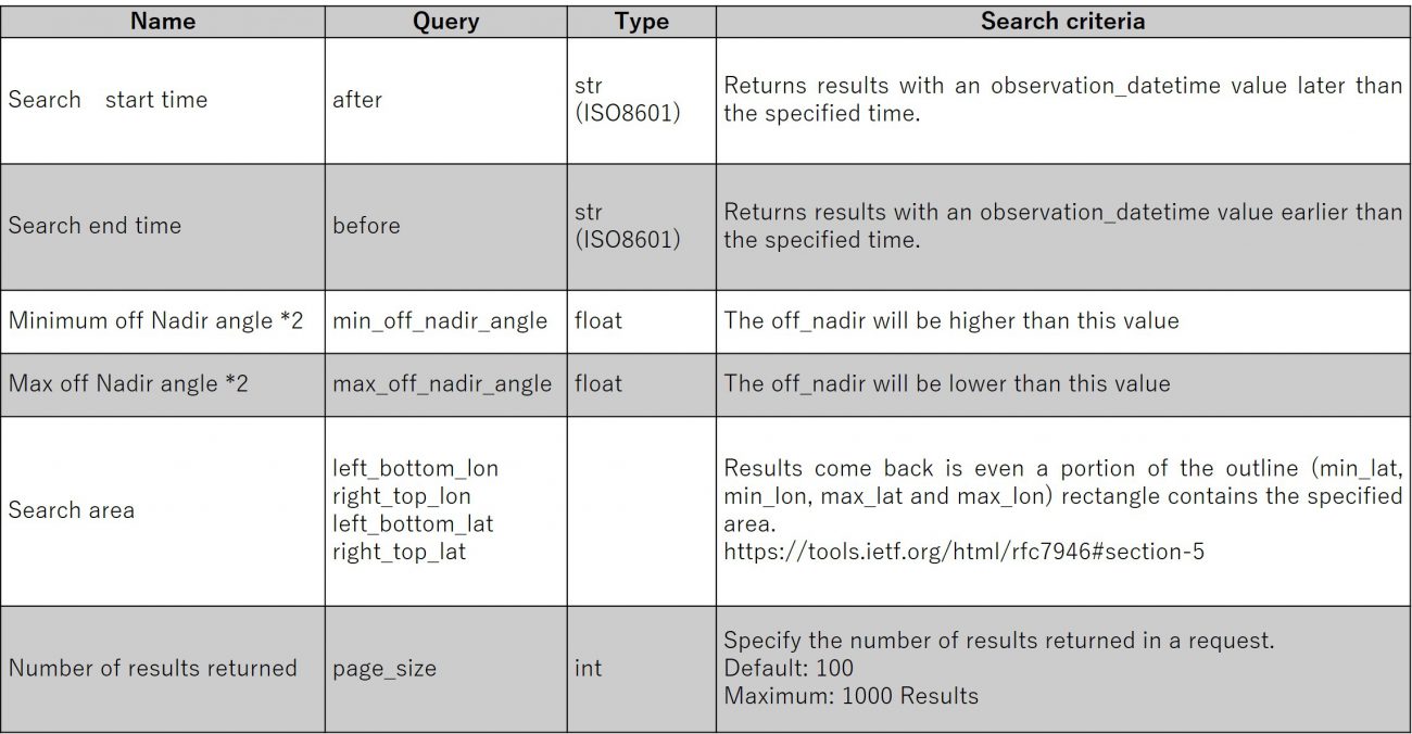

*1 RSP is short for Reference System for Planning. You can think of it as a search system.
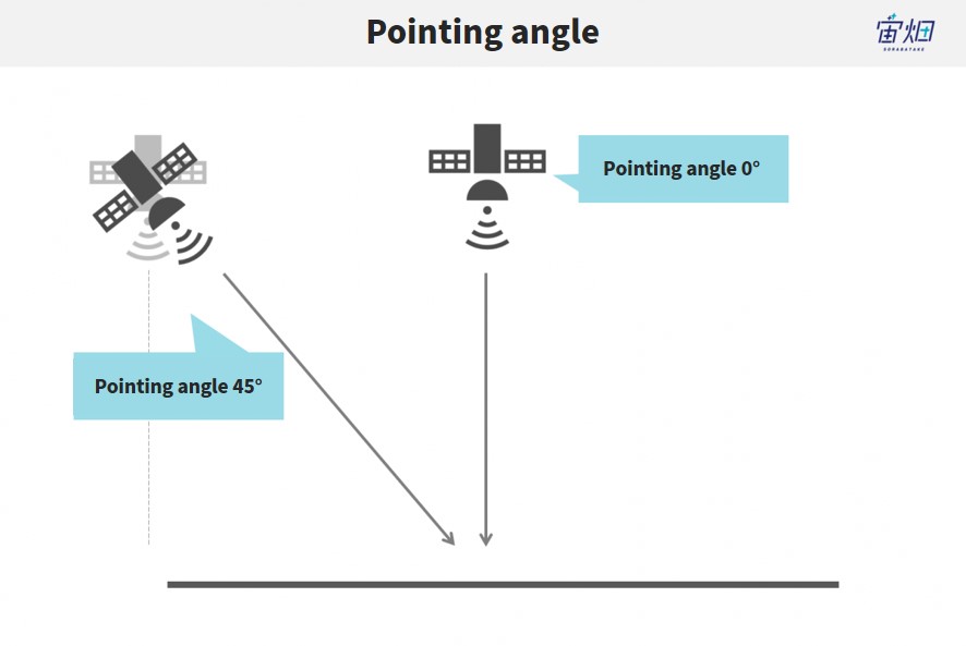
*2 Pointing Angle:
the angle at which the photo is taken. Use 0 deg. for taking pictures from directly above, and 90 deg. for taking pictures directly from the side.

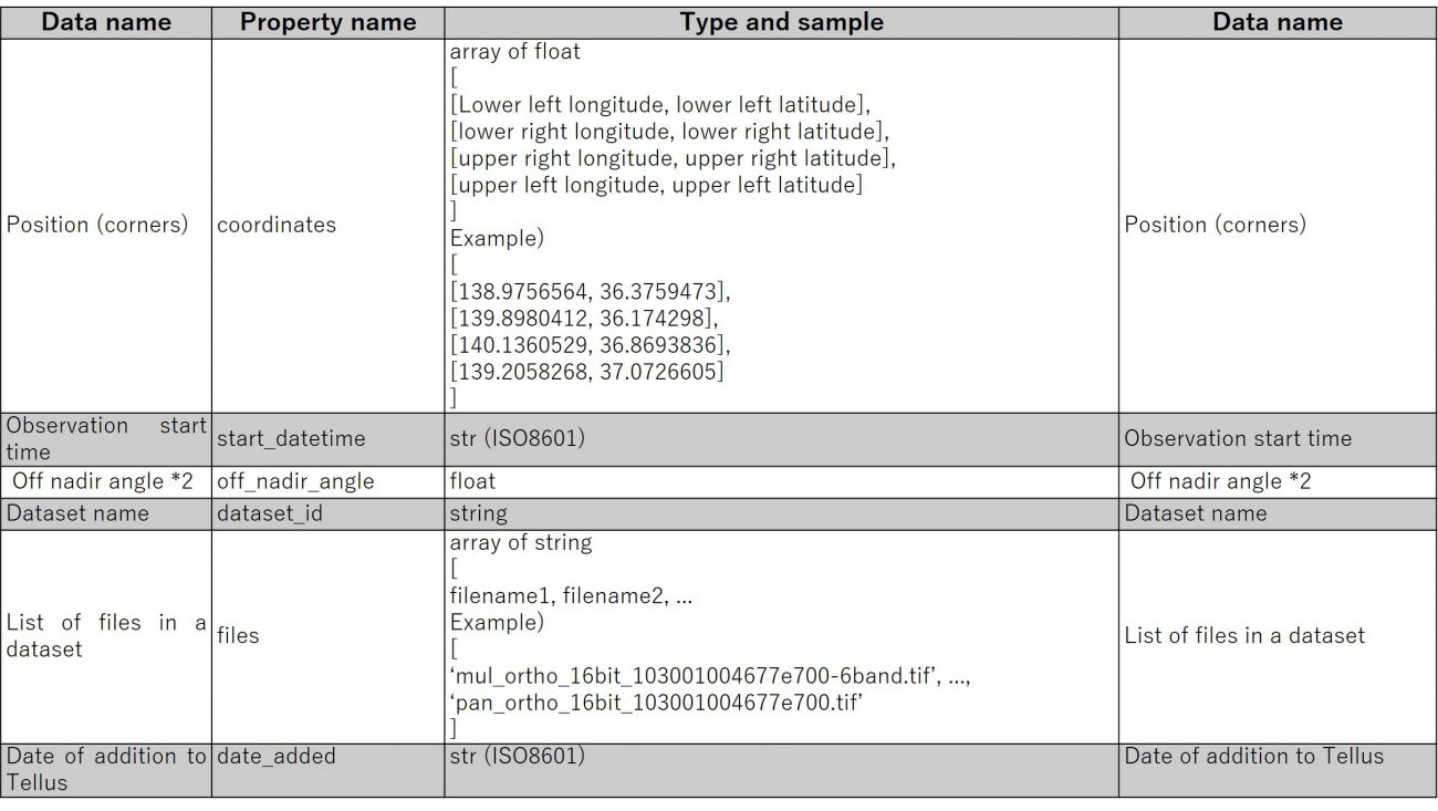
Return value

1. Do a file search

First, create a method for running the file search API.
Please log into your My Page, and obtain a token from the access settings (this requires logging in).

import os, requests
import pprint

TOKEN = 'ここには自分のアカウントのトークンを貼り付ける'
DOMAIN = 'tellusxdp'

# ファイル検索メソッド
def search_file(params={}, next_url=''):
    if len(next_url) > 0:
        url = next_url
    else:
        url = f"https://file.{DOMAIN}.com/api/v1/origin/search/alos3-pseudo"
    
    headers = {
        'Authorization': f"Bearer {TOKEN}"
    }
    r = requests.get(url, params=params, headers=headers)
    if not r.status_code == requests.codes.ok:
        r.raise_for_status()
    return r.json()

This function receives a dictionary of parameters and then returns the content of header text of corresponding files in JSON format.

Let’s try searching for a file.
We will be using the following search criteria this time.
– Three results in a request

# サンプル1
# 雲量10%以下 かつ ポインティング角が20deg以下、一度に取得する件数は3件
metas = search_file({'page_size': 3})
# 検索結果を表示
pprint.pprint(metas)

When you run the code, it will show you the output below.

{'count': 3,
 'items': [{'bbox': [130.1990675, 33.4411108, 130.3169171, 33.7018372],
            'coordinates': [[130.1990675, 33.4411108],
                            [130.3169171, 33.4411108],
                            [130.3169171, 33.7018372],
                            [130.1990675, 33.7018372]],
            'dataset_id': 'alos3-pseudo_ortho_1030010040c36f00',
            'date_added': '2020-08-25T07:10:36.524131',
            'files': ['ObsDate.txt',
                      'pan_ortho_16bit_1030010040c36f00_1.tif',
                      'pan_ortho_16bit_1030010040c36f00_2.tif',
                      'mul_ortho_16bit_1030010040c36f00_1-6band.tif',
                      'mul_ortho_16bit_1030010040c36f00_2-6band.tif'],
            'observation_datetime': '2015-04-18T02:25:02.841574+00:00',
            'off_nadir_angle': 27.45,
            'publish_link': 'https://file.tellusxdp.com/api/v1/origin/publish/alos3-pseudo/alos3-pseudo_ortho_1030010040c36f00',
            'start_datetime': '2015-04-18T02:25:02.841574+00:00',
            'type': 'a'},
           {'bbox': [130.2833888, 33.4926222, 130.4611712, 33.615915],
             <2件目省略>
           },
           {'bbox': [130.3150367, 33.5071697, 130.4953247, 33.7129745],
             <3件目省略>
           }],
 'next': 'https://file.tellusxdp.com/api/v1/origin/search/alos3-pseudo?cursor=eyJjdXJzb3JfbGFzdF90aW1lIjogIjIwMTYtMDMtMTdUMDI6MDg6MTAuMzEwMTE5IiwgImN1cnNvcl9iZWdpbl90aW1lIjogIjIwMTUtMDQtMThUMDI6MjU6MDIuODQxNTc0IiwgInN0YXJ0X3RpbWUiOiAiMTk3MS0wMS0wMVQwMDowMDowMCIsICJlbmRfdGltZSI6ICIyMDIwLTA5LTE0VDEyOjEzOjA0LjUxNzI1NyJ9'}

A URL with the key called “next” is displayed at the end of the output.

This URL allows you to see the rest of the results when there are too many that match the criteria to acquire in a single search, or when you have set a maximum number of results.

Next, let’s use the URL to acquire the remaining result.

# サンプル2
# 同じ条件で続きを取得する、取得件数を1件にする
metas = search_file({'page_size': 1}, next_url = metas['next'])
pprint.pprint(metas)

Below is the output.

{'count': 1,
 'items': [{'bbox': [138.1604347, 36.5139777, 138.3189499, 36.7656609],
            'coordinates': [[138.1604347, 36.5139777],
                            [138.3189499, 36.5139777],
                            [138.3189499, 36.7656609],
                            [138.1604347, 36.7656609]],
            'dataset_id': 'alos3-pseudo_ortho_104001001d101e00',
            'date_added': '2020-08-25T07:10:36.524131',
            'files': ['ObsDate.txt',
                      'pan_ortho_16bit_104001001d101e00.tif',
                      'mul_ortho_16bit_104001001d101e00-6band.tif'],
            'observation_datetime': '2016-06-03T01:42:30.433484+00:00',
            'off_nadir_angle': 28.3,
            'publish_link': 'https://file.tellusxdp.com/api/v1/origin/publish/alos3-pseudo/alos3-pseudo_ortho_104001001d101e00',
            'start_datetime': '2016-06-03T01:42:30.433484+00:00',
            'type': 'b'}],
 'next': 'https://file.tellusxdp.com/api/v1/origin/search/alos3-pseudo?cursor=eyJjdXJzb3JfbGFzdF90aW1lIjogIjIwMTYtMDYtMDNUMDE6NDI6MzAuNDMzNDg0IiwgImN1cnNvcl9iZWdpbl90aW1lIjogIjIwMTYtMDYtMDNUMDE6NDI6MzAuNDMzNDg0IiwgInN0YXJ0X3RpbWUiOiAiMTk3MS0wMS0wMVQwMDowMDowMCIsICJlbmRfdGltZSI6ICIyMDIwLTA5LTE0VDEyOjEzOjA0LjUxNzI1NyJ9'}

We got another result for the same condition.

Normally you would filter your search to get the results you desire, but there isn’t much data to filter yet, so we will skip that for now.
For readers who are interested in this data, read our article on AVNIR-2.

2. Acquire the download URL

You can download result files to see the actual data.
To do this, you need to get the URLs used for downloading the files.

Make a function to get the URLs used for downloading the files.

def publish_file(dataset_id='', searched_url=''):
    if len(searched_url) > 0:
        url = searched_url
    else:
        url = 'https://file.{}.com/api/v1/origin/publish//publish/alos3-pseudo/{}'.format(DOMAIN, dataset_id)
    
    headers = {
        'Authorization': 'Bearer ' + TOKEN
    }

    r = requests.get(url, headers=headers)
    if not r.status_code == requests.codes.ok:
        r.raise_for_status()
    return r.json()

Run the function to get the download URLs.

Using the file search method from earlier, let’s try and acquire a URL from the data at the top of the search results.

# サンプル4
# 取得用URL発行（検索結果から取得したい場合）
# ファイル検索
metas = search_file({'page_size': 10})
# ダウンロードURL発行
published = publish_file(searched_url=metas['items'][0]['publish_link'])
# 結果を表示する
pprint.pprint(published)

Once you’ve done this, it should look like the following.

{'dataset_id': 'alos3-pseudo_ortho_1030010040c36f00',
 'expires_at': '2020-09-15T00:20:54.585179+00:00',
 'files': [{'file_name': 'ObsDate.txt',
            'file_size': 1883,
            'url': 'https://file.tellusxdp.com/api/v1/origin/eyJ0eXAiOiJKV1QiLCJhbGciOiJIUzI1NiJ9.eyJpYXQiOjE2MDAwODYwNTQsImV4cCI6MTYwMDEyOTI1NCwiYXBpX3Rva2VuIjoiMGRmOGE4ZmJmNGE5IiwiZGF0YXNldCI6ImFsb3MzLXBzZXVkbyIsImtleSI6ImFsb3MzLXBzZXVkb19vcnRob18xMDMwMDEwMDQwYzM2ZjAwIiwiZmlsZV9uYW1lIjoiT2JzRGF0ZS50eHQifQ.TBz5DH0lBU6VKg_EGEH9nht_vKvt-gtREai441X2BVw'},
           {'file_name': 'mul_ortho_16bit_1030010040c36f00_1-6band.tif',
            'file_size': 427820635,
            'url': 'https://file.tellusxdp.com/api/v1/origin/eyJ0eXAiOiJKV1QiLCJhbGciOiJIUzI1NiJ9.eyJpYXQiOjE2MDAwODYwNTQsImV4cCI6MTYwMDEyOTI1NCwiYXBpX3Rva2VuIjoiMGRmOGE4ZmJmNGE5IiwiZGF0YXNldCI6ImFsb3MzLXBzZXVkbyIsImtleSI6ImFsb3MzLXBzZXVkb19vcnRob18xMDMwMDEwMDQwYzM2ZjAwIiwiZmlsZV9uYW1lIjoibXVsX29ydGhvXzE2Yml0XzEwMzAwMTAwNDBjMzZmMDBfMS02YmFuZC50aWYifQ.JS3AH_41bSvpceoo6wuGrQziLCshwhXKFnAluDKHDI4'},
            <省略>

           ],
 'project': 'alos3-pseudo'}

The “files” array has the name (file_name), size (file_size) and download URL (url) of each file.

“url” contains the URL to download the file from.

This URL expires after a certain time, which is assigned to expires_at. After this time, the URL becomes invalid and you will need to get another URL.

3. Download the Files

Start by establishing the method with which you’ll download the files.

def download_file(url, dir, name):
    headers = requests.utils.default_headers()
    headers["Authorization"] = "Bearer " + TOKEN

    r = requests.get(url, headers=headers, stream=True)
    if not r.status_code == requests.codes.ok:
        r.raise_for_status()
    if os.path.exists(dir) == False:
        os.makedirs(dir)
    with open(os.path.join(dir,name), "wb") as f:
        for chunk in r.iter_content(chunk_size=1024):
            f.write(chunk)

Next, download the file using the URL you acquired from the file above.

for file in published['files']:
    if re.match(r'.*tif$', file['file_name']):
        pprint.pprint(file['file_name'])
        download_file(file['url'], published['dataset_id'], file['file_name'],)

It takes some time due to the size of the file.

4. Display the image

Now, let’s read and show one of the downloaded GeoTiff files.

import numpy as np
import rasterio as rio
import matplotlib.pyplot as plt
from skimage.exposure import rescale_intensity

file_name = "mul_ortho_16bit_103001004677e700-6band.tif"
src_file = f"{published['dataset_id']}/{file_name}"
with rio.open(src_file) as src:
    bands = src.read()
    
bgr = np.dstack((bands[1,:,:], bands[2,:,:], bands[3,:,:]))
p_low, p_high = np.percentile(bgr,(0,99.5))
bgr_8bit = rescale_intensity(bgr,in_range=(p_low, p_high), out_range=(0,255)).astype(np.uint8)
plt.imshow(bgr_8bit)
plt.show()

Doing this should show you an image like the one below.

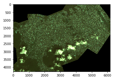
If you wish to save the image, run the following code.

import cv2
cv2.imwrite("hogehoge.png", bgr_8bit)

All 6 wavelengths of the mock ALOS-3 data can be found in the files starting with “mul”.
ALOS-3 contains the
band 1: coastal
band 2: blue
band 3: green
band 4: red
band 5: red edge
band 6: NIR
settings.
(data details: http://www.satnavi.jaxa.jp/project/alos3/)
The sample code from above shows color images synthesized from bands 2, 3, and 4.

The band settings are as follows.

This time we are working with color images, so for blue we used band 2 (blue), for green we used band 3 (green), and red we used band 4 (red).

And that brings us to the end of our introduction on how to acquire the mock ALOS-3 data on Tellus’ development environment.

Now’s your chance to try fiddling around with the data before the real ALOS-3 launches into space.

★Register for Tellus here