[How to Use Tellus from Scratch] Get data from the Automated Meteorological Data Acquisition System (AMeDAS) on JupyterLab
You can get observed data values at one-minute intervals of rain, anemometers, thermometers, sunshine recorders and snow gauges of the Automated Meteorological Data Acquisition System (AMeDAS) on Tellus. In this post, we'll show you how to get this AMeDAS data using JupyterLab on Tellus.
In this post, we’ll show you how to get data from the Automated Meteorological Data Acquisition System (AMeDAS) using JupyterLab on Tellus.
Please refer to “API available in the developing environment of Tellus” for how to use Jupyter Lab (Jupyter Notebook) on Tellus.
1. Get AMeDAS data using the API
You can get one-minute data (observation data at one-minute intervals) of AMeDAS using the API on Tellus.
For how to use an API, it is summarized in this reference.
API reference
*Please make sure to check the data policy (Data Details)not to violate the terms and conditions when using data.
https://gisapi.tellusxdp.com/api/v1/amedas/1min/{yyyy}/{MM}/{dd}/{hh}/{mm}/{?min_lat,min_lon,max_lat,max_lon}Input details
| yyyy | Required str |
Observation year in the Gregorian calendar (in a four-digit format) *UTC Example: ‘2016’ |
| MM | Required
str |
Observation month; 01 – 12 (in a two-digit format) *UTC Example: ’01’ |
| dd | Required str |
Observation date; 01 – 31 (in a two-digit format) *UTC Example: ’01’ |
| hh | Required str |
Observation hour; 00 – 23 (in a two-digit format) *UTC Example: ’12’ |
| mm | Required
str |
Observation minute; 00 – 59 (in a two-digit format) *UTC Example: ’00’ |
| min_lat | Optional
number |
Minimum latitude of monitoring stations(−90.0 – 90.0) |
| min_lon | Optional number |
Minimum longitude of monitoring stations (−180.0 – 180.0) |
| max_lat | Optional
number |
Maximum latitude of monitoring stations (−90.0 – 90.0) |
| max_lon | 任意 number |
Maximum longitude of monitoring stations (−180.0 – 180.0) |
*Data from December 31, 2015 to December 31, 2017 in UTC is available on Tellus at this time.
Let’s call up this API from Notebook on Jupyter Lab.
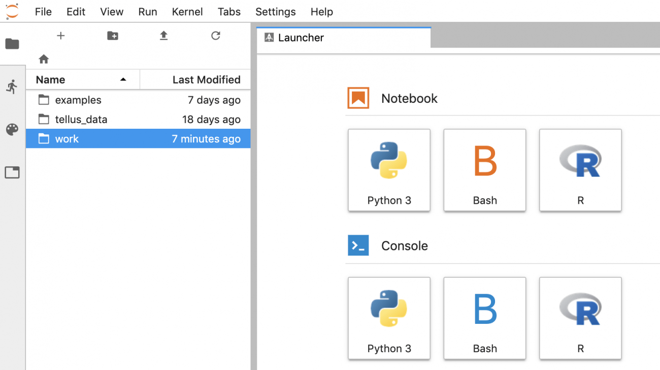
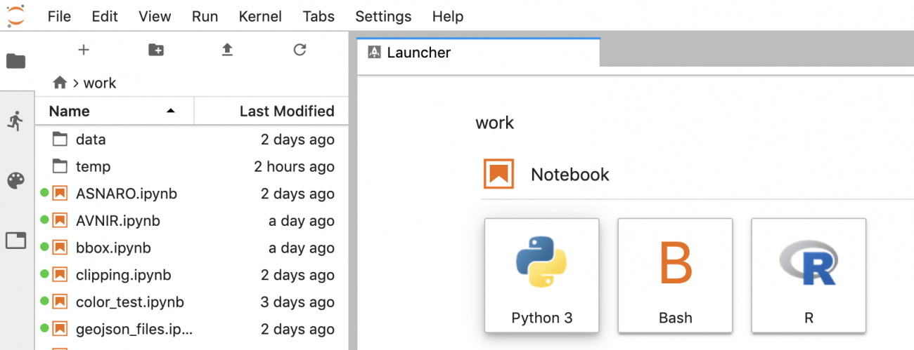
Open Tellus IDE, go to the “work” directory, select “Python 3,” and paste the following code.
import requests, json

TOKEN = 'ここには自分のアカウントのトークンを貼り付ける'

def get_amedas_1min(year, month, day, hour, minute, payload={}):
    """
    /api/v1/amedas/1minを叩く

    Parameters
    ----------
    year : string
        西暦年 (4桁の数字で指定) UTC
    month : string
        月 01~12 (2桁の数字で指定) UTC
    day : string
        日 01~31 (2桁の数字で指定) UTC
    hour : string
        時 00~23 (2桁の数字で指定) UTC
    minute : string
        分 00~59 (2桁の数字で指定) UTC
    payload : dict
        パラメータ(min_lat,min_lon,max_lat,max_lon)

    Returns
    -------
    content : list
        結果
    """

    url = 'https://gisapi.tellusxdp.com/api/v1/amedas/1min/{}/{}/{}/{}/{}/'.format(year, month, day, hour, minute)

    headers = {
        'Authorization': 'Bearer ' + TOKEN
    }
    r = requests.get(url, headers=headers, params=payload)

    if r.status_code is not 200:
        print(r.content)
        raise ValueError('status error({}).'.format(r.status_code))
    return json.loads(r.content)

amedas1 = get_amedas_1min('2015', '12', '31', '15', '01')
print(len(amedas1))
print(amedas1[0])
Get the token from APIアクセス設定 (API access settings) in My Page (login required).
Click the triangle icon at the top to run the code. Data for the specified time will be presented.
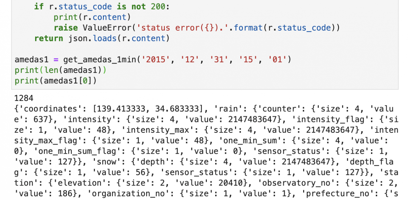
The sample code gets data for 00:01 on January 1, 2016 Japan time.
You get one request to obtaim data of all the monitoring stations in Japan for the specified time.
It says there were 1,284 monitoring stations as of January 2016.
The API returns observation time, coordinates (latitude & longitude), monitoring station information, rain gauge data, anemometer data, thermometer data, sunshine recorder data and snow gauge data.
The structure of each observed value is like this:
{
    "value": int,
    "size": int
}
For observations from which the sensors didn’t give data, the maximum value in the byte length (size) is assigned to the value. (Example: {“size”: 4, “value”: 2147483647})
You can narrow the range of data you need by using the latitude and longitude function.
payload = {
    'min_lat': 39.0,
    'min_lon': 139.0,
    'max_lat': 40.0,
    'max_lon': 140.0
}
amedas2 = get_amedas_1min('2015', '12', '31', '15', '01', payload)
print(len(amedas2))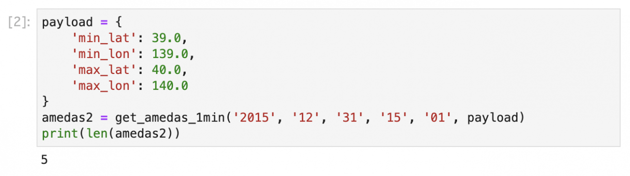
The sample code requests data for longitude 139° – 140° and latitude 39° – 40°. Data of five monitoring stations within this range is available.
2. Rain gauge data
Rain gauge data consists of observed values such as precipitation during the preceding minute, intensity and maximum intensity; and the flags indicate quality of data.
Let’s sort the top 10 intensity values in descending order and display them.
We get data observed at 17:30 on October 28, 2017 Japan time. Data with the default value (2147483647) or 12 or more quality flags (which indicates bad observation quality) are excluded as error values in this sample.
def is_valid(value_obj, flag_obj):
    byte_size = {
        1: 127,
        2: 32767,
        4: 2147483647
    }
    return flag_obj['value'] <= 12 and value_obj['value'] != byte_size[value_obj['size']]

amedas2 = get_amedas_1min('2017', '10', '28', '8', '30')
amedas2_sorted = sorted(amedas2, key=lambda d: d['rain']['intensity']['value'], reverse=True)
amedas2_filtered = list(filter(lambda d: is_valid(d['rain']['intensity'], d['rain']['intensity_flag']), amedas2_sorted))

for i in range(10):
    print('station_id : ' + str(amedas2_filtered[i]['station']['prefecture_no']['value']).zfill(2) + str(amedas2_filtered[i]['station']['observatory_no']['value']).zfill(3)
          + ', intensity : ' + str(amedas2_filtered[i]['rain']['intensity']['value']/10) + '[mm/h]')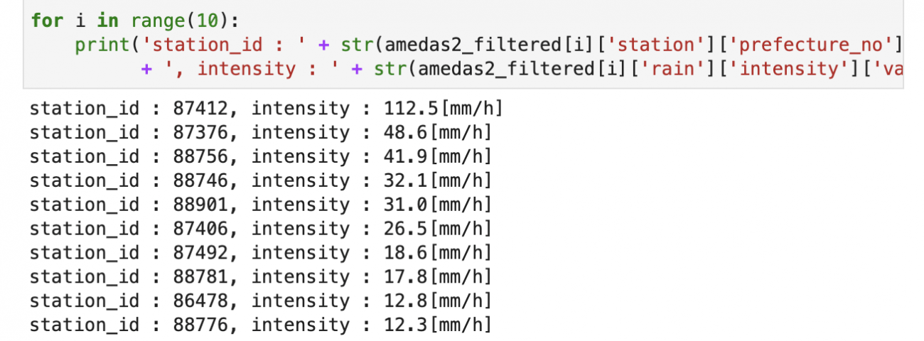
Station #87412 — Akae Station in Miyazaki prefecture — took the top spot with the highest intensity in Japan.
You can say rain with an intensity of 112.5 mm/h like this is quite heavy as precipitation of more than 50 mm/h is referred to as a downpour.
Monitoring stations ranked second or below are all located in Kyushu. Why is this? Because the Typhoon Saola was approaching Kyushu aty that time.
3. Anemometer data
Anemometer data consists of observed values such as maximum instantaneous wind velocity (three-second moving average), average wind velocity (10-minute moving average) and average wind direction (vector average during the preceding 10 minutes); and flags that indicate quality of data.
Let’s observe how the average wind velocity (velocity_ave) and the average wind direction in 16 directions (direction_ave_16direction) change as a typhoon approaches.
We get hourly data for the period when Typhoon Saola was passing by western Japan (24 hours of data from 21:00 on October 28), from one monitoring station located in southwestern Shikoku – the Shimizu Special Automated Weather Station (station #74516).
Data with the default value (2147483647) or with 12 or more quality flags (which indicates bad observation quality) are excluded as error values in this sample.
from datetime import datetime
from datetime import timedelta

direction_label = ['無風',
                   '北北東', '北東', '東北東', '東',
                   '東南東', '南東', '南南東', '南',
                   '南南西', '南西', '西南西', '西',
                   '西北西', '北西', '北北西', '北',]

time = datetime(2017,10,28,21,0,0) - timedelta(hours=9)
for i in range(24):
    amedas_3 = get_amedas_1min(str(time.year), str(time.month).zfill(2), str(time.day).zfill(2), str(time.hour).zfill(2), str(time.minute).zfill(2))
    amedas_91011 = next(d for d in amedas_3 if str(d['station']['prefecture_no']['value']).zfill(2) + str(d['station']['observatory_no']['value']).zfill(3) == '74516')

    if is_valid(amedas_91011['wind']['velocity_ave'], amedas_91011['wind']['velocity_ave_flag']):
        print(amedas_91011['timestamp'], '{}[m/s]'.format(amedas_91011['wind']['velocity_ave']['value']/10), direction_label[amedas_91011['wind']['direction_ave_16direction']['value']])

    time += timedelta(hours=1)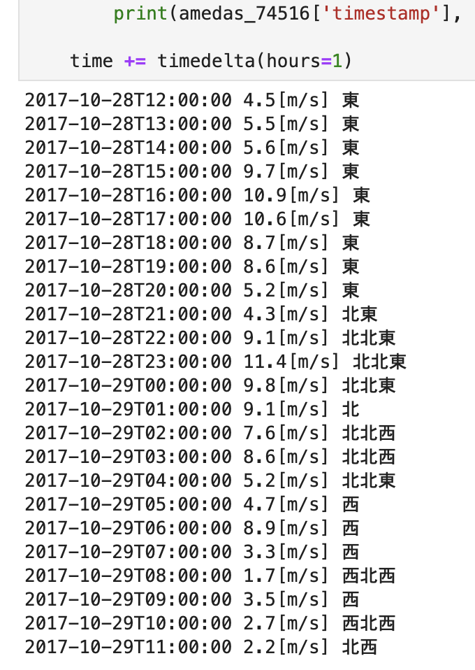
Typhoon Saola passed the southern coast of Shikoku from west to east. The observation data confirms that the wind direction changed from east to north to west as the typhoon went by the region, with winds blowing toward the center of the typhoon.
4. Thermometer data
Thermometer data consists of observed values such as temperature, maximum temperature (during the preceding minute) and minimum temperature (during the preceding minute); and flags that indicate quality of data.
Let’s make graphs of temperatures at three of the hottest recorded spots in Japan — from the Kumagaya Local Meteorological Observatory (station #43056), the Ekawasaki Weather Station (station #74381) and also the Tajimi Weather Station (station #52606) — and put the graphs together.
We get hourly data from 0:00 to 24:00 on August 1, 2016 Japan time. Data with the default value (2147483647) or with 12 or more quality flags (which indicates bad observation quality) are excluded as error values in this sample.
import matplotlib.pyplot as plt
import matplotlib.dates as mdates
%matplotlib inline

time = datetime(2016,8,1,0,0,0) - timedelta(hours=9)

kumagaya = []
egawa = []
tajimi = []
periods = []

for i in range(24):
    amedas_4 = get_amedas_1min(str(time.year), str(time.month).zfill(2), str(time.day).zfill(2), str(time.hour).zfill(2), str(time.minute).zfill(2))
    # 熊谷
    amedas_43056 = next(d for d in amedas_4 if str(d['station']['prefecture_no']['value']).zfill(2) + str(d['station']['observatory_no']['value']).zfill(3) == '43056')
    # 江川崎
    amedas_74381 = next(d for d in amedas_4 if str(d['station']['prefecture_no']['value']).zfill(2) + str(d['station']['observatory_no']['value']).zfill(3) == '74381')
    # 多治見
    amedas_52606 = next(d for d in amedas_4 if str(d['station']['prefecture_no']['value']).zfill(2) + str(d['station']['observatory_no']['value']).zfill(3) == '52606')

    if is_valid(amedas_43056['temperature']['deg'], amedas_43056['temperature']['deg_flag']):
        kumagaya.append(amedas_43056['temperature']['deg']['value']/10)
    else:
        kumagaya.append(0)
    if is_valid(amedas_74381['temperature']['deg'], amedas_74381['temperature']['deg_flag']):
        egawa.append(amedas_74381['temperature']['deg']['value']/10)
    else:
        egawa.append(0)
    if is_valid(amedas_52606['temperature']['deg'], amedas_52606['temperature']['deg_flag']):
        tajimi.append(amedas_52606['temperature']['deg']['value']/10)
    else:
        tajimi.append(0)
    periods.append(time + timedelta(hours=9))
    time += timedelta(hours=1)

fig, ax= plt.subplots(figsize=(12, 6))
ax.plot(periods, kumagaya, label = 'no marker')
ax.plot(periods, egawa, label = 'no marker')
ax.plot(periods, tajimi, label = 'no marker')
ax.legend(['kumagaya', 'egawa', 'tajimi'])
xfmt = mdates.DateFormatter('%H')
xloc = mdates.HourLocator()
ax.xaxis.set_major_locator(xloc)
ax.xaxis.set_major_formatter(xfmt)
ax.set_xlabel('hour(JST)')
ax.set_ylabel('temp')
ax.set_xlim(periods[0], periods[-1])
plt.show()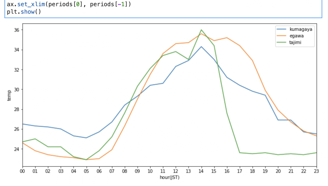
Tajimi was the hottest of the three on this day.
This is how you get data from the Automated Meteorological Data Acquisition System (AMeDAS) using JupyterLab on Tellus.
AMeDAS one-minute data is a gigantic data set that has more than 600 million records for each year. What about using this wonderful set of statistics and data with high temporal resolution to complement your satellite data?