Types of Satellite Orbit: Orbits, Trajectories, and Routes for Travel
The Final Instalment of a Three-Part Series on Artificial Satellite Orbits: Exploring Commonly Used Orbits for Satellites
In the previous two instalments, we introduced artificial satellite orbits. In this final article, we will showcase several commonly used types of orbits.
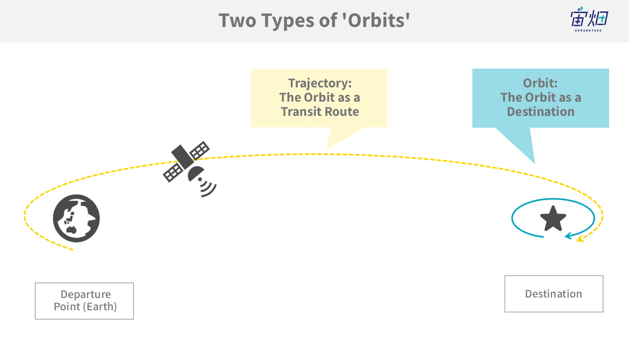
We will begin by introducing the destination ‘Orbit’. This is the orbit of the satellite around the target and to get to this orbit, we will need to travel via a certain ‘Trajectory’.
Orbit types
There are various orbit types depending on the various factors such as mission requirements, observation requirements, communication, local environment, etc.
For instance, in the case of Earth observation satellites, there might be a requirement to pass over a specific location in Japan at a particular time in JST under similar solar incidence conditions.
To meet such demands, specific orbits (such as the Sun-Synchronous Orbit, which will be discussed later) need to be chosen as destinations. Let’s now take a visual tour of these orbits as destinations.
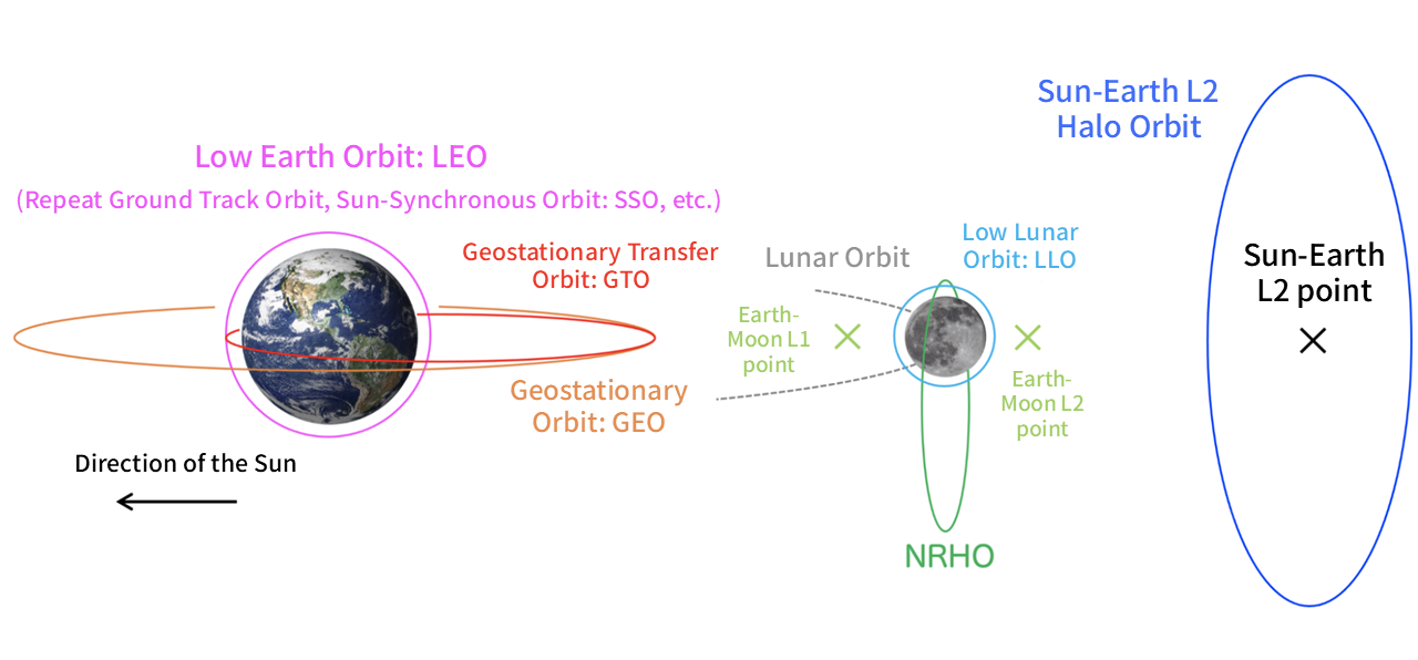
Low Earth Orbit (LEO)
Currently, the most common orbit utilised for satellites is the Low Earth Orbit (LEO). Generally, it refers to orbits below 2000 km altitude from the Earth’s surface. Depending on the altitude, it can be further classified into Medium Earth Orbit (MEO) and High Earth Orbit (HEO), but LEO is the most widely used for Earth observation due to its practicality.
The International Space Station (ISS) also orbits in LEO. Within LEO, there are two particularly popular types of orbits: “Repeat Ground Track Orbit” and “Sun-Synchronous Orbit”.
Repeat Ground Track Orbit (RGT) and Quasi-Periodic Orbit
A Repeat Ground Track Orbit is an orbit in which a satellite completes exactly N orbits around Earth in the time it takes for Earth to complete one rotation on its axis. This means that the satellite will pass over the same point on Earth’s surface at approximately the same time each day.
A related orbit is the Quasi-Periodic Orbit, where a satellite completes N orbits around Earth in the time it takes for Earth to complete M rotations. This means that while the satellite doesn’t pass over the same point on Earth’s surface every day, it will do so every M days.
These orbits are popular for missions like Earth observation and communication because they allow for regular and predictable coverage of specific areas on Earth.
Sun-Synchronous Orbit (SSO)
Another popular orbit is the Sun-Synchronous Orbit (SSO). The term “Sun-Synchronous Orbit” refers to an orbit where the orientation of a satellite’s orbital plane remains consistent with respect to the sun over the course of a year. This orbit takes advantage of the fact that the Earth is not a perfect sphere but rather a slightly flattened ellipsoid.
Because the orientation of the satellite’s orbital plane relative to the sun remains constant throughout the year, SSO allows for consistent lighting conditions for Earth observation. This ensures that the satellite captures images under nearly identical lighting conditions each day.
One additional advantage of the Sun-Synchronous Orbit is that the periods of shadowing (when the satellite is in the Earth’s shadow) remain relatively constant throughout the year.
By selecting a well-designed Sun-Synchronous Orbit, it’s even possible to achieve an orbit with continuous exposure to sunlight, referred to as a “Dawn-Dusk Orbit.” This means that the satellite experiences sunlight without interruption.
This orbit type is advantageous not only for consistent lighting conditions but also from a power and thermal design perspective. It’s a popular choice for Synthetic Aperture Radar (SAR) satellites, which require substantial power.
There also exist orbits that combine Sun-Synchronous characteristics with those of Repeat Ground Track or Near-Repeat orbits. These orbits are highly favoured for missions in Low Earth Orbit (LEO).
Furthermore, orbits like Low Lunar Orbit (LLO) and Low Mars Orbit are widely utilised for missions to the Moon and Mars, respectively. The feasibility of setting up practical Repeat Ground Track orbits or SSO in these orbits depends on the rotational period and gravitational characteristics of the celestial body in question.
Geostationary Orbit (GEO)
In missions like communication and weather observation, one of the most popular orbits is the Geosynchronous Equatorial Orbit, also referred to as a Geostationary Orbit, commonly known as GEO.
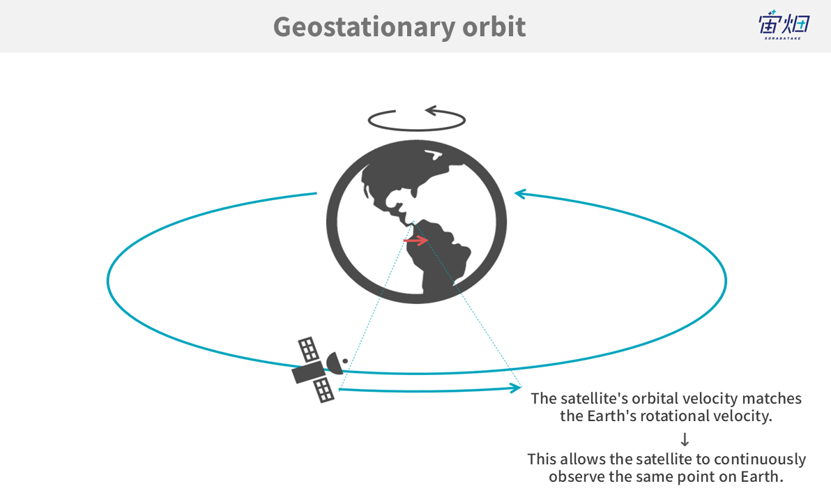
The GEO is a circular orbit located at an altitude of approximately 35,786 kilometres above the Earth’s surface, with an inclination angle of 0 degrees (directly above the equator). In this orbit, a satellite’s orbital period matches the Earth’s rotational period. Consequently, the satellite remains fixed over the same point on the Earth’s surface at all times.
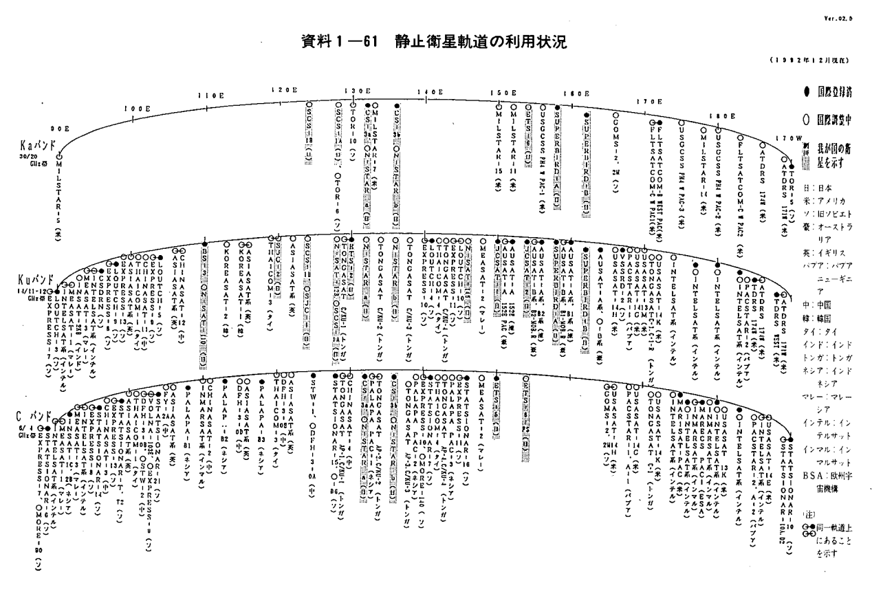
Source : https://www.soumu.go.jp/johotsusintokei/whitepaper/ja/h05/html/h05b0161.html
GEO is particularly favoured for a wide range of applications, including the continuous monitoring of one’s own country from space, weather observation, and communication missions. Due to the limited capacity for satellites in GEO and the inherent challenges associated with its higher altitude, larger and more versatile satellites with extended lifespans are the predominant choice compared to satellites in lower orbits.
This orbit has played a crucial role in various fields of space-based applications, and its popularity continues to grow with ongoing advancements in technology and the increasing demand for real-time and high-bandwidth communication services.
Geosynchronous Orbit (GSO) and Quasi-Zenith Orbit
GEO is a type of Geosynchronous Orbit (GSO). In GSO, the satellite’s orbital period aligns with the Earth’s rotation period. There are no specific constraints regarding orbital inclination angle or eccentricity.
While a satellite in GSO doesn’t stay directly above a single point on the Earth’s surface, it remains in close proximity to a particular point. A quasi-zenith orbit, exemplified by the deployment of the “Michibiki” quasi-zenith satellite, is a specific type of orbit within the GSO category.
For positioning satellites, it’s considered advantageous to distribute satellites across the celestial sphere over the desired locations to enhance positioning accuracy. By choosing a quasi-zenith orbit, satellites can be stationed above Japan while being spread out across the sky over Japan.
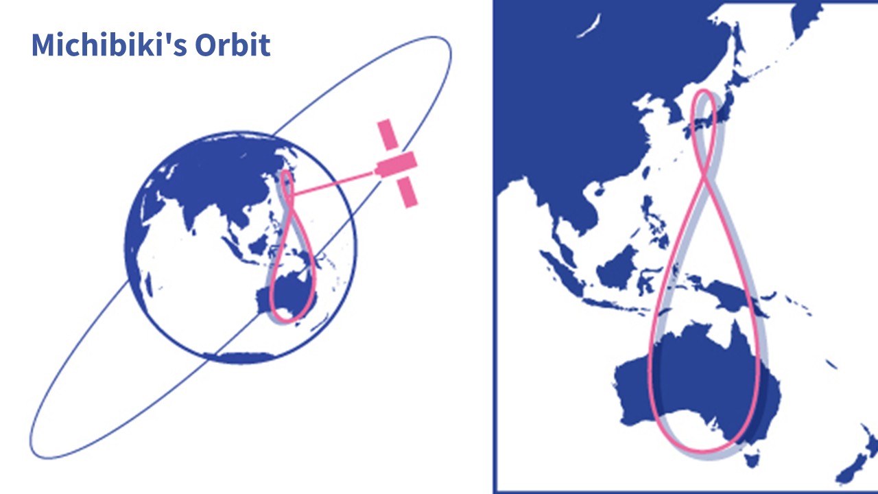
Quasi-zenith orbits have proven crucial for enhancing the accuracy and availability of positioning services, particularly in regions with complex topography or urban environments where signals from conventional satellites may be obstructed. The Michibiki system, being one of the pioneers in this category, significantly contributes to Japan’s positioning capabilities and augments global navigation systems.
Halo Orbit
For missions extending beyond Earth’s orbit towards the Moon and beyond, a special type of orbit called the Halo Orbit is employed.
Currently, there is a surge in missions targeting regions beyond the Moon, spurred by developments like the Lunar Orbital Platform-Gateway (LOP-G) and NASA’s Artemis program. The landscape of space business is gradually transitioning from Earth-centric orbits to regions extending beyond the Moon.
The proposed base for these missions is the Near Rectilinear Halo Orbit (NRHO), which is a subtype of the “Halo Orbit” based on the concept of “Lagrangian Points.” To begin, let’s delve into explanations of both “Lagrangian Points” and “Halo Orbits.”
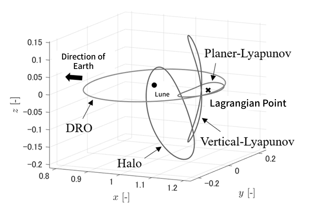
Lagrangian Points
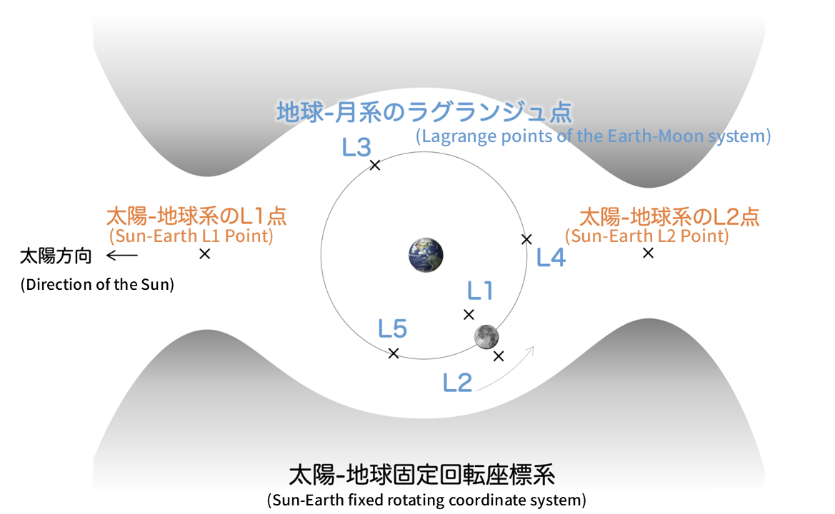
Lagrangian Points refer to the dynamic equilibrium points (where forces are balanced) that exist in the three-body problem (for instance, Sun-Earth-Spacecraft, Earth-Moon-Spacecraft, etc.). With near equilibrium near these points, these points can be utilised as ‘parking spots’ for spacecraft to remain in a fixed position while consuming minimal fuel.
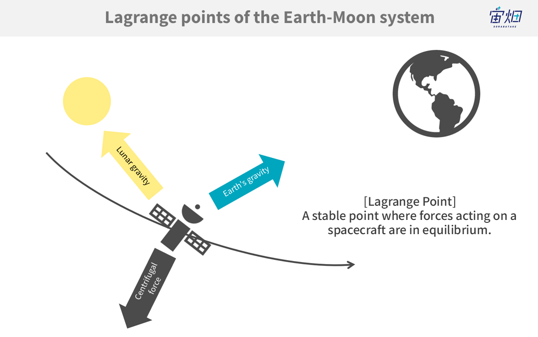
For instance, in the Earth-Moon system’s Lagrangian Points, the gravitational forces exerted by the Earth and the Moon, along with the centrifugal force, are balanced, resulting in these dynamic equilibrium points.
Given that multiple points of equilibrium exist, these points are denoted as L1, L2, L3, and so forth, with reference to Lagrange (L), who introduced this concept. Specifically, L1 and L2 in the Sun-Earth system are often utilised for missions such as solar observation (for continuous observation of the Sun) and astronomical satellites (for continuous observation while protecting telescopes from solar heat), respectively. For example, L2 in the Earth-Moon system provides high accessibility to both Earth and the far side of the Moon, enabling communication between them. This is why it’s been chosen as a potential site for the Lunar Orbital Gateway.
It’s important to note that this refers to the Circular Restricted Three-Body Problem (CR3BP), where one of the bodies, such as a spacecraft, is significantly smaller than the other two (in this case, the Earth and the Moon).
Halo Orbit
Since Lagrangian Points are merely points of equilibrium, when positioning spacecraft, they are placed in periodic orbits near these points.
Among the various periodic orbits near Lagrangian Points, the most famous is the Halo Orbit.
Credit : Takuya Chikazawa, University of Tokyo
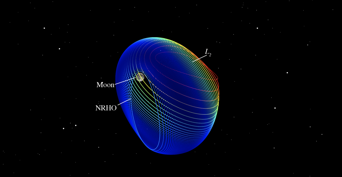
Different Halo Orbits exist for each energy level of the orbit, and among these, the Near Rectilinear Halo Orbit (NRHO) refers to Halo Orbits that closely resemble long, elliptical orbits passing near the Moon.
The proposed Lunar Orbital Gateway is planned to be located in the NRHO of the Earth-Moon L2 point.
The Orbit as a Transit Route
Up to this point, we’ve discussed the destination ‘Orbits’. Now, let’s talk about orbits as transit routes: the Transfer Orbit or Trajectory.
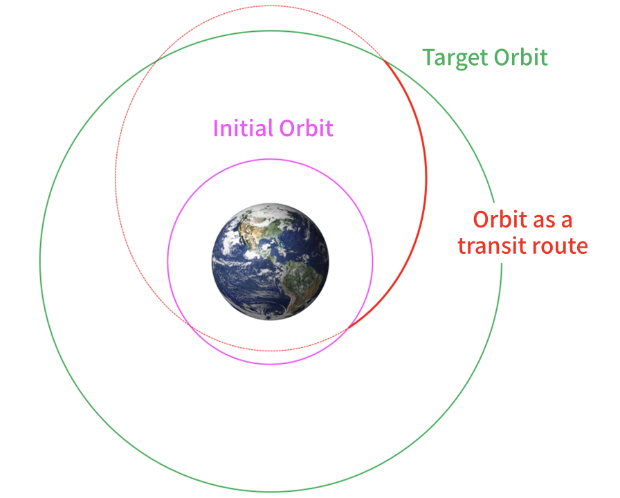
To move from an initial orbit to a target orbit, one simply needs to select a Transfer Orbit which intersects (i.e., aligns positions) with both of these initial and target orbits.
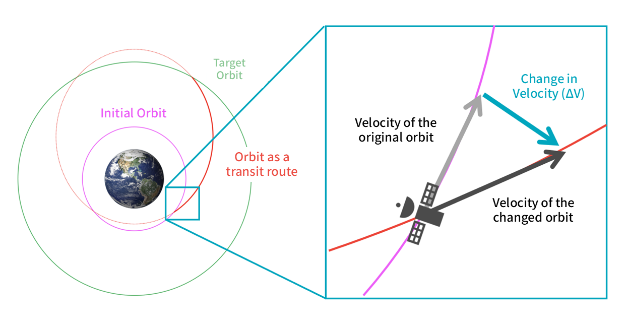
Transitioning from the initial orbit to the transfer orbit involves adjusting velocity at the point where these orbits intersect. This adjustment is known as ΔV (Delta V). ΔV is calculated as the difference in velocity (vector).
Then, at the point where the transfer orbit and the target orbit intersect, another velocity adjustment allows you to reach the desired orbit.
There are typically multiple options for such transit routes. Therefore, choosing the best orbit from these various routes is crucial for mission success. This is where the expertise in “orbit optimization” comes into play.
The criteria for selecting the best orbit vary depending on the mission, but often involve choosing an orbit that minimises the fuel consumption of the rocket or spacecraft.
Calculation of Fuel Consumption for Orbit Change
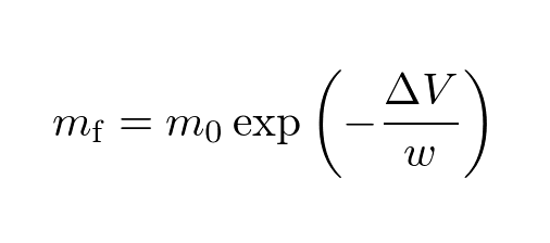
The fuel consumption of a rocket can be calculated using Tsiolkovsky’s Rocket Equation. The derivation of Tsiolkovsky’s Rocket Equation is covered in various textbooks, so we’ll skip it here.
Effective exhaust velocity is a measure of a rocket’s performance; the higher it is, the more efficient the rocket. For example, for solid rockets, it’s around 2.45 km/s, for liquid rockets, about 3.43 km/s, and for ion engines like the one famous from the Hayabusa mission, it’s around 29.4 km/s! Developing a rocket with a high is one of the research challenges for rocket propulsion researchers.
Now, let’s use a Jupyter notebook to calculate the mass that a rocket can carry. To barely escape from Low Earth Orbit (LEO) to deep space, about 3.3 km/s of V is needed (calculated from the difference between the second cosmic velocity, 11.2 km/s, and the first cosmic velocity, 7.9 km/s). Assuming an initial mass of 1000 kg for a liquid rocket, let’s calculate the mass it can carry from LEO to deep space.
import numpy as np
dv = 3.3 # ΔV from LEO to deep space, km/s
w = 3.43 # Effective exhaust velocity of the liquid rocket, km/s
m0 = 1000 # Initial mass, kg
mf = m0*np.exp(-dv/w) print(mf)
This means that if we use a 1000 kg liquid rocket, about 60% (618 kg, calculated as 1000 kg – 382 kg) of it will be consumed as fuel! Note that the remaining mass of 382 kg includes rocket propulsion hardware, tanks, and supporting structures, so caution is necessary. This should give you an understanding of how important the size of V and is.
Now, let’s introduce a few methods for calculating V. However, actual V calculations are very complex, so this will be an introductory level. If you want to study in more detail, refer to books or other resources. In the following, we assume a two-body problem for all cases.
Hohmann transfer orbit
The Hohmann Transfer Orbit, known as the orbit with the minimum ΔV, is recognized when both the initial and target orbits are circular and lie in the same plane.
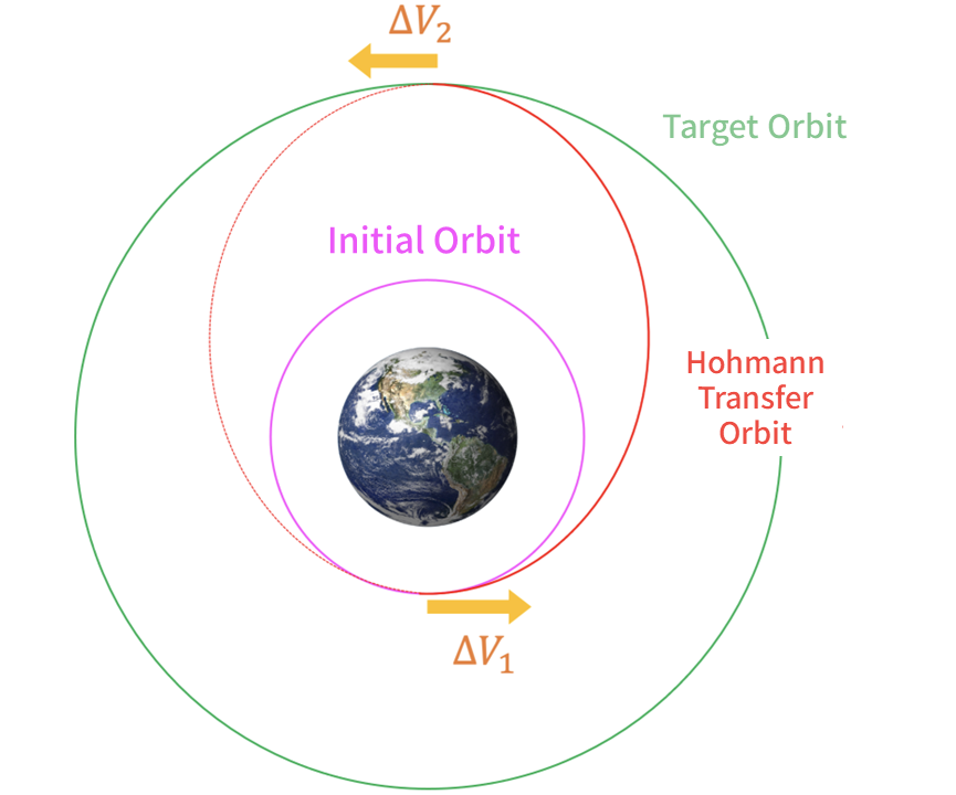
The intuitive explanation for why the Hohmann transition orbit has a ΔV minimum is that it is more efficient for the satellite to give ΔV in the direction of travel. Regardless of the Hohmann transition orbit, it is often more efficient to give ΔV in the direction of velocity.
If the perigee radius of the ellipse is denoted as rp and the apogee radius is denoted as ra, the velocity at the perigee and apogee of the ellipse can be calculated using the following equation:
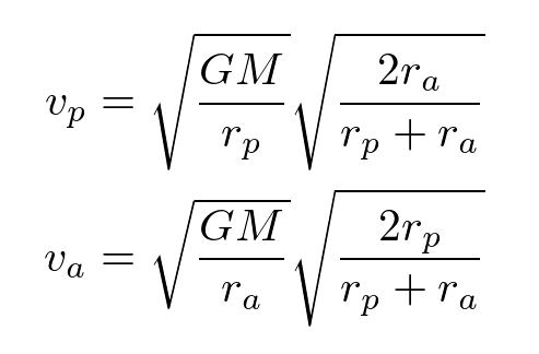
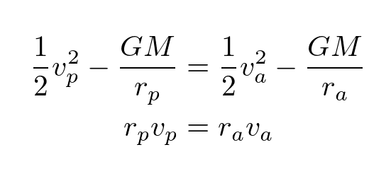
It’s worth mentioning that these formulas are derived from the conservation of energy and angular momentum in elliptical orbits.
Now, let’s calculate the required ΔV to transition from a Low Earth Orbit (LEO) with a radius of 6778 km to a Geosynchronous Orbit (GEO) with a radius of 42164 km using a Jupyter Notebook:
import numpy as np

# Given data
GM = 398600.4354360959  # Earth's gravitational constant, km^3/s^2
rp = 6778  # Radius of LEO, km
ra = 42164  # Radius of GEO, km

# Velocities of LEO and GEO orbits
v_LEO = np.sqrt(GM / rp) * np.sqrt(2 * rp / (rp + rp))  # Both periapsis and apoapsis are rp in a circular orbit
v_GEO = np.sqrt(GM / ra) * np.sqrt(2 * ra / (ra + ra))  # Both periapsis and apoapsis are ra in a circular orbit

# Velocities for Hohmann Transfer Orbit
vp = np.sqrt(GM / rp) * np.sqrt(2 * ra / (rp + ra))
va = np.sqrt(GM / ra) * np.sqrt(2 * rp / (rp + ra))

# Calculate ΔVs
dv1 = vp - v_LEO
dv2 = v_GEO - va

print(dv1, dv2)
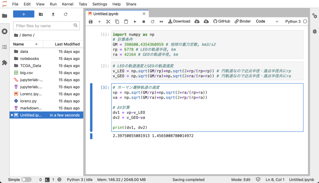
The transfer from a Low Earth Orbit to Geosynchronous Orbit is known as a Geostationary Transfer Orbit (GTO). The calculated ΔV1 is usually handled by the rocket, and ΔV2 is designed to be carried out by the satellite. To determine how much fuel is needed for the satellite to achieve the required ΔV2 of 1.46 km/s, you can calculate it using the rocket equation.
The Lambert Problem
The Hohmann Transfer Orbit was applicable under the condition that both the initial and target orbits were circular and lay in the same plane. However, in reality, many orbits do not meet these criteria.
One widely used method among experts for calculating transitions between orbits is solving the “Lambert Problem.”
The Lambert Problem addresses the calculation of initial and final velocities given the initial and final positions, as well as the transition time.
Here’s the input-output relationship for the Lambert Problem:
input-output relationship for the Lambert Problem
|
Input
|
Output
|
|
Initial Position Final Position Transition Time |
Initial Velocity Final Velocity |
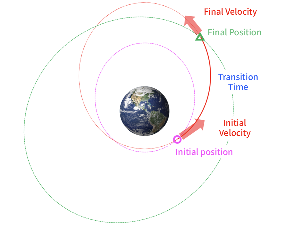
The theory behind the Lambert Problem requires hours to explain in detail. Therefore, we’re presenting only the results here.
Now, let’s use a Jupyter Notebook to solve the Lambert Problem. If pykep is not already installed, you’ll need to install it.
import pykep as pk
import numpy as np

# Given data
GM = 398600.4354360959  # Earth's gravitational constant, km^3/s^2
r1 = np.array([0.01, -6778.0, 0.0])  # Position in LEO, km
r2 = np.array([0.01, 42164.0, 0.0])  # Position in GEO, km
tof = 19048.4026989538  # Half of GTO orbital period, s

# Solve the Lambert Problem
l = pk.lambert_problem(r1=r1, r2=r2, tof=tof, mu=GM)

# Calculate ΔV
v_LEO = np.sqrt(GM / 6778.0)  # Velocity in LEO, km/s
v_GEO = np.sqrt(GM / 42164.0)  # Velocity in GEO, km/s
v1 = l.get_v1()[0]  # Initial velocity calculated from Lambert Problem
v2 = l.get_v2()[0]  # Final velocity calculated from Lambert Problem
dv1 = abs(v1[0]) - v_LEO
dv2 = v_GEO - abs(v2[0])

print(dv1, dv2)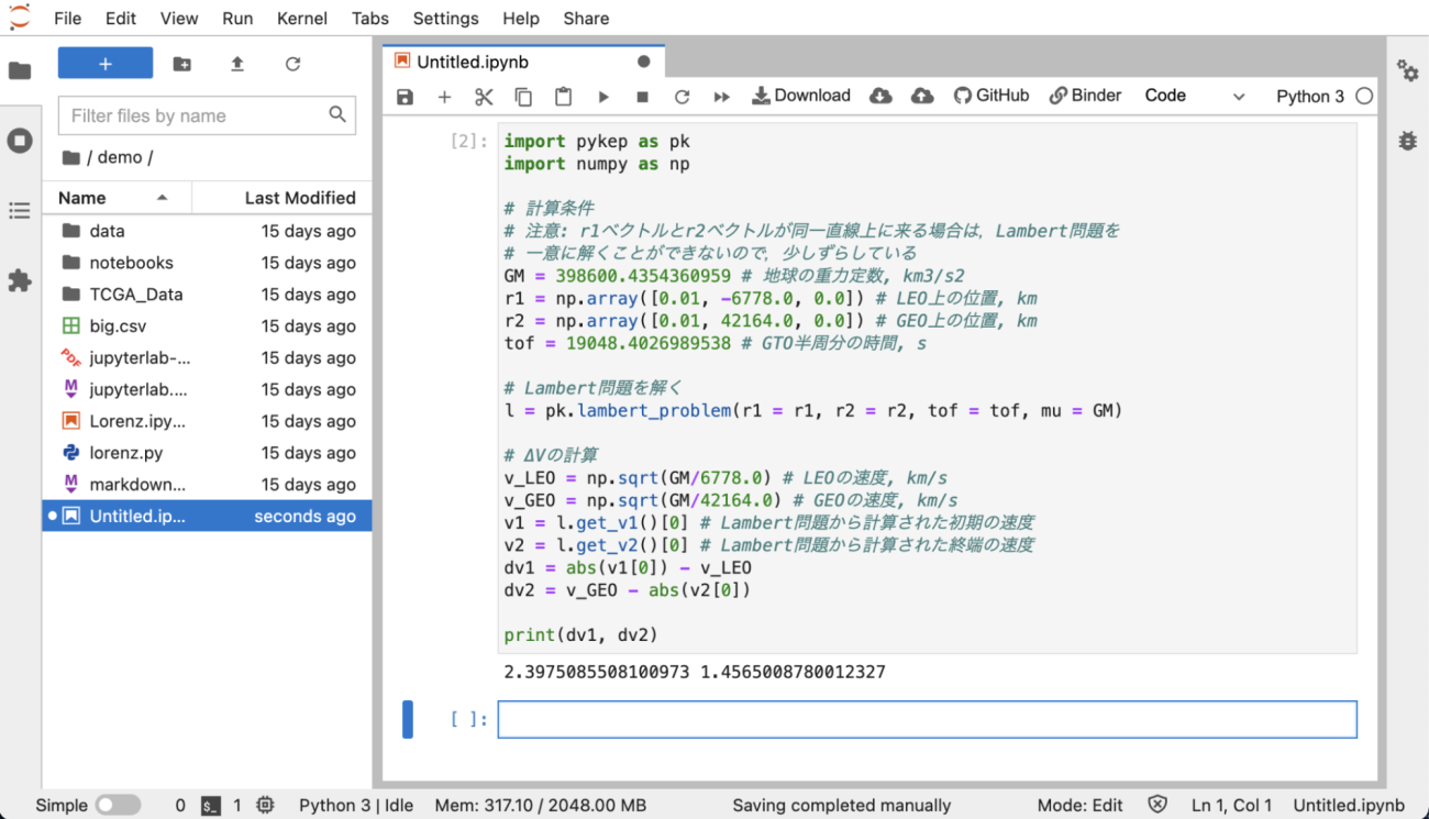
Did you get results similar to those calculated using the Hohmann Transfer Orbit? Solving the Lambert Problem allows us to compute more general transition orbits. It’s important to note that the Lambert Problem does not compute the “optimal” transition orbit from the initial to the target orbit. To find the optimal transition orbit, you would need to explore orbits by varying the initial and final positions as well as the transition time.
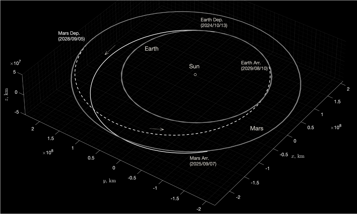
In JAXA’s Martian Moons eXploration (MMX) project for Earth-to-Mars orbit transitions, the Lambert Problem is employed. However, when dealing with celestial bodies like Earth or Mars, one must consider the effect of the gravitational bending of orbits near these bodies. The “Patched Conics” approach is often used for such problems.
Future Prospects
In this article, we’ve explained satellite and spacecraft orbits from two perspectives: “Destination Orbits” and “Transfer Orbits”. While we didn’t touch on it in this article, orbit analysis (primarily using orbit propagation) is essential for evaluating whether space debris might collide with other satellites and for estimating when it will re-enter the Earth’s atmosphere in the coming years. This article provided an introductory discussion on orbits, but calculating favourable orbits for missions and efficient transition orbits requires more advanced knowledge.
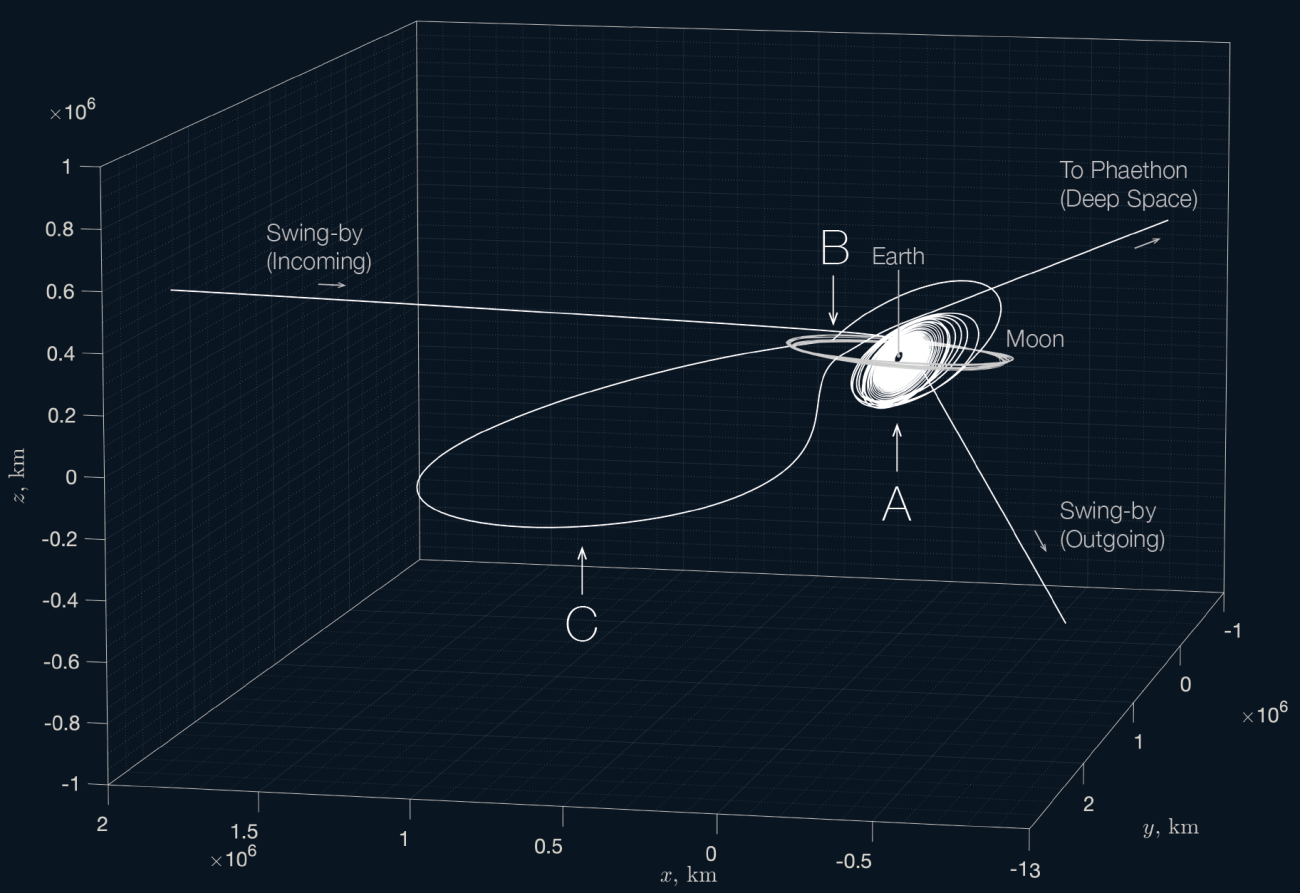
For example, in the 2020s, JAXA aims to launch the deep space exploration technology demonstrator DESTINY+, which combines the spiral orbit control using ion engines developed in projects like Hayabusa and Hayabusa2 with the lunar multi-swing-by technique used in missions like Kaguya and NOZOMI. This combination is expected to enable deep space exploration even with small rockets, paving the way for a new era in space exploration.
When it comes to travelling on Earth, the widespread use of car navigation systems and tools like Google Maps in recent years has made it possible to travel without detailed planning. However, space travel currently requires the expertise of orbital specialists to determine destinations and transit routes. As the Artemis program and the Lunar Gateway project lead to the expansion of space utilisation and space business, I believe the demand for expertise in orbital matters will continue to grow. I hope this article sparks interest in orbits among many readers.