It is cold outside. Around this time of year, I feel like going snowboarding, taking a break from working on a computer. Going snowboarding every winter, I have realized each ski area has different snow conditions every year, including hard-packed, heavy, or even no snow.

If satellite data can be used to estimate snow conditions, it might help in arranging a schedule that allows me to find a ski area with the best snow conditions to snowboard.

In this article, snow conditions will be analyzed using satellite data on Tellus in the future.
The newly released satellite data platform, Tellus, is compatible with Jupyter Notebook, a useful tool for Python data analysis. Since the API on Tellus is now available, we would like to introduce some functions of Jupyter Notebook by analyzing snow conditions.

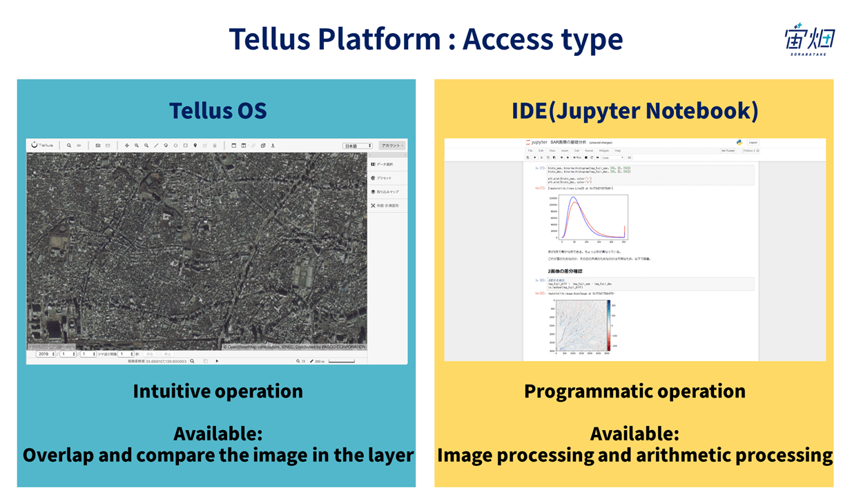
There are two major ways of accessing Tellus. One is Tellus OS, which allows you to put multiple data on a map in a Web-browser, and the other is developing an environment where programming is used for data analysis (hereafter called Jupyter Notebook).

In the developing environment of Tellus, various data and Jupyter Notebook are connected through API. You can use and analyze data using programmed API.

(1) Start Jupyter Notebook

Please refer to the following URL for setting up Jupyter Notebook on Tellus.
https://www.tellusxdp.com/ja/tutorial

First, sign up for Tellus.

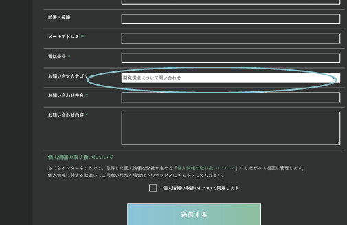
As it says “Please make an inquiry from the contact form,” select “Questions regarding the development environment for Cloud and High-end servers.” from the Inquiry category on the contact form, write “I would like to use Jupyter Notebook environment,” and send the form.

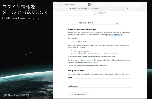
After that, the office will send you an email, asking you to send your Tellus account information.

Then, you will receive your login information for Jupyter Notebook. Set your initial password and log in to the development environment. Follow the explanation written in the email for logging in the future.

Log in to Tellus OS while staying logged in on Jupyter Notebook and click the terminal icon located in the upper left. Click “Open Jupyter Notebook.”

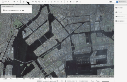
Then, Jupyter Notebook top page will appear.

(2) Look at the default directories on Jupyter Notebook

Logging in to the Jupyter Notebook environment, you will see some directories. Each directory is composed of the following elements:

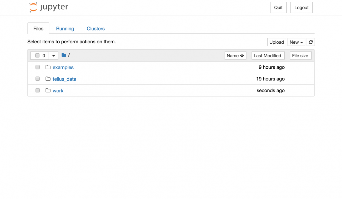
●/examples: It has a sample code that cannot be edited. You can use this code for snow condition analysis.

●/tellus_data: It is a directory that stores data sent from Tellus OS to Jupyter Notebook. This article explains how to send data from Tellus OS. Sent as a tiff as the data cannot be displayed in Jupyter Notebook for now.

●/work: It is a directory that you can create your own notebook. You can also import notebooks.

Since directories other than work are read only, all the documents you newly create or update are saved under the work directory.

In addition to the pre-installed basic library, you can install additional libraries using pip and conda commands by opening Terminal in the New tab.

*However, directories except for work, tellus_data, and their subordinates, may be reset due to updates. Therefore, we recommend you to write down what you have got.

(3) How to analyze

Next, we will look at the usable satellite data on Tellus.
Data Catalog｜Tellus

To consider various ski slopes in the future, the most suitable optical image would be AVNIR-2(ALOS) or Landsat. Synthetic Aperture Radar (SAR), which can obtain images behind the cloud using microwave, is also helpful because optical images are not always available when it is snowing (as snow is covered with cloud). PALSAR-1(ALOS) and PALSAR-2(ALOS-2) are the recommended SAR images as they cover the entire of Japan.

However, since AVNIR-2 is the only open API in Tellus at this moment, we would like to use AVNIR-2 for the analysis. *In the Jupyter Notebook environment, some of the satellite images of PALSAR-2 are also available as sample data.

(4) Obtain images using API

Now we are going to obtain images using API. The following is the list of APIs to be updated.
API Reference｜Tellus

We are going to acquire optical images around Mt. Fuji from Tellus. AVNIR-2 data is obtained from the optical sensor installed on the Advanced Land Observing Satellite Daichi (ALOS). A visible light image, just like what humans can see, can be created by synthesizing images within the blue, green, and red light wavelength bands.

The following article explains wavelength in detail.

What is light wavelength? Why satellites can see things not visible to the human eye?

You can actually use the snow conditions analysis example to follow each step from obtaining API to the analysis. To deepen your understanding, you may want to open the sample file while reading the following explanation.

When you open the examples directory, you will find the following composing elements. First, please make sure to read README.md. The notebooks directory contains notebooks on both optical and SAR codes for snow condition analysis. The data directory stores the data used for this analysis.

README.md：It explains the overall composition of this sample.

/notebooks：Both optical and SAR Python codes for snow condition analysis are stored.

/data：Data used for this analysis is stored.

You can specify a location to retrieve data as follows:

(*Internal API is used in the sample code.)

 # Domain of API
URL_DOMAIN = "https://gisapi.opf-dev.jp/"

# Location of Mt.Fuji
Z = 13
X = 7252
Y = 3234

def get_data(img_type, domain=URL_DOMAIN, z=Z, x=X, y=Y):
    return io.imread("{}/{}/{}/{}/{}.png".format(domain, img_type, z, x, y))

# Open Street Map as Base Map
img_osm = get_data("osm")
# Satellite Data
img_band1= get_data("av2ori/band1")
img_band2 = get_data("av2ori/band2")
img_band3 = get_data("av2ori/band3")
img_band4 = get_data("av2ori/band4")

(5) Start analysis!

The following sample code performs various basic analyses using images. This article covers snow segmentation as a basic optical image analysis.

Caution:
Some of the Tellus APIs used in this notebook are especially created for sample use. They are subject to change without notice.

The analysis procedures in this article are not based on academic knowledge but are the results confirmed as the possible changes in the images, thus accuracy is not guaranteed.

mport numpy as np
from skimage import io
from skimage import color
from skimage import img_as_ubyte
from skimage import filters
import matplotlib.pyplot as plt
%matplotlib inline

Acquisition and preparation of optical images

We are going to obtain optical images taken around Mt. Fuji from Tellus. Tiled PNG data is used for this analysis. XYZ method is adopted to specify the location. Please click here (external website) for more information.

The following example uses data obtained through a sensor called AVNIR-2 in ALOS. For more information on AVNIR-2, please click here (external website).

Caution:

The APIs used here are for sample use only. It can only be used within the Tellus Jupyter environment.  Official APIs are scheduled to be released in the future.

# Domain of API
URL_DOMAIN = "https://gisapi.opf-dev.jp/"

# Location of Mt.Fuji
Z = 13
X = 7252
Y = 3234

def get_data(img_type, domain=URL_DOMAIN, z=Z, x=X, y=Y):
   return io.imread("{}/{}/{}/{}/{}.png".format(domain, img_type, z, x, y))

img_osm = get_data("osm")
img_band1= get_data("av2ori/band1")
img_band2 = get_data("av2ori/band2")
img_band3 = get_data("av2ori/band3")
img_band4 = get_data("av2ori/band4")

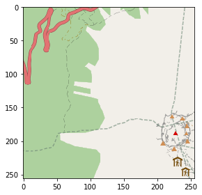
Confirmation of OpenStreetMap

Since it is difficult to determine the specified location only from the satellite images, prepare the information on OpenStreetMap to use as a reference.

print(img_osm.shape)
io.imshow(img_osm)
(256, 256, 3)

When the code above is executed, you will get the following result.

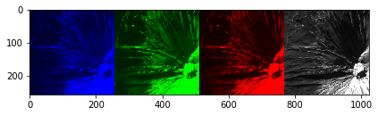
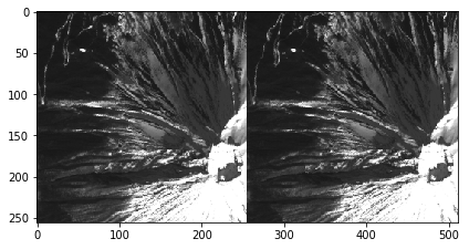
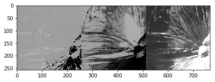
Confirmation of AVNIR-2

Data of four different wavelengths can be used in AVNIR-2. Generally, Band 1, Band 2, Band 3, and Band 4 correspond to blue, green, red, and near-infrared wavelengths respectively. The following code is used to see individual wavelength.

io.imshow(np.hstack((img_band1,img_band2,img_band3,img_band4)))

The following is the result of the code execution.

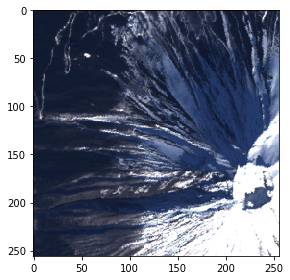
Since each image corresponds to blue, green, red (and near-infrared) visible light, the composite image of RGB (Red-green-blue) looks like what the human eye can see. This composite image is called true color image.

RGB composite of true color

●R: Band3（red）
●G: Band2（green）
●B: Band1（blue）

The following code is used to create true color image.

img_true = np.c_[img_band3[:,:,0:1], img_band2[:,:,1:2], img_band1[:,:,2:3]]
io.imshow(img_true)

The following is the result of the code execution.

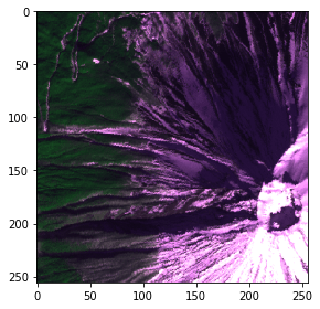
There are also other composite methods. For example, the natural color composite, in which plant distribution area is colored in green, is used when you want to emphasize only regions of the vegetation. Utilizing the high reflection rate of near-infrared light, red color is assigned to the red wavelength (Band3), green color to the near-infrared wavelength (Band4), and blue color to the green wavelength (Band2).

RGB composite of natural color

●R: Band3（red）
●G: Band4（near-infrared）
●B: Band2（green）

The following code is used to create natural color image.

img_natural = np.c_[img_band3[:,:,0:1], img_band4[:,:,0:1], img_band2[:,:,1:2]]
io.imshow(img_natural)

The following is the result of the code execution.

Intuitive detection of snow using whitish color

Now, let’s detect snow.

We are going to extract snow based on the intuition that whitish part of the mountain represents snow. First, create a grayscale image from the true color one, using two methods, then try to extract snow by determining the threshold.

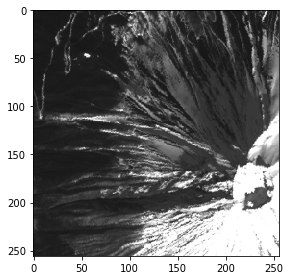
Determination of snow by grayscaling Grayscaling ①

Grayscaling ①
Try to directly create a grayscale image using skimage.color.rgb2gray. The code is as follows.

#Convert color image to Grayscale image
img_gray_01 = color.rgb2gray(img_true)

# Change the value range ([0, 1] -> [0, 255])
img_gray = img_as_ubyte(img_gray_01)

print("Before Conversion: [0, 1]")
print(img_gray_01)
print("After Conversion: [0, 255]")
print(img_gray)

io.imshow(img_gray)
Before Conversion: [0, 1]
[[ 0.10348667  0.10629216  0.09759294 ...,  0.13229098  0.4027102
   0.28838863]
 [ 0.10993098  0.10432     0.10712549 ...,  0.12278118  0.33378078
   0.18417294]
 [ 0.09675961  0.10320392  0.10684275 ...,  0.11662745  0.33016471
   0.21639373]
 ..., 
 [ 0.10853922  0.10825647  0.1090898  ...,  1.          1.          1.        ]
 [ 0.10714039  0.10825647  0.1090898  ...,  1.          1.          1.        ]
 [ 0.11189529  0.11441804  0.11189529 ...,  1.          1.          1.        ]]
After Conversion: [0, 255]
[[ 26  27  25 ...,  34 103  74]
 [ 28  27  27 ...,  31  85  47]
 [ 25  26  27 ...,  30  84  55]
 ..., 
 [ 28  28  28 ..., 255 255 255]
 [ 27  28  28 ..., 255 255 255]
 [ 29  29  29 ..., 255 255 255]]

You can obtain the following image after the code execution. It is certainly a well grayscaled image.

Grayscaling ②
Let’s try another grayscaling method. Convert RGB color space into YIQ color space. Since the grayscale information is separated from the color data in the YIQ format, you can use the same signal for both colors, black and white.

(*img_gray_01 and img_yiq[:, :, 0] may become equal in some grayscaling algorithms, but not in skimage.)

The following is the code.

img_yiq = color.rgb2yiq(img_true)
img_conb = np.concatenate(
   (img_yiq[:, :, 0], img_yiq[:, :, 1], img_yiq[:, :, 2]), axis=1)
io.imshow(img_conb)

Here is the result.

Let us compare the grayscaled images created using two methods. The code used for comparison is as follows.

# Compare with “skimage.color.rgb2gray”
img_conb2 = np.concatenate((img_yiq[:, :, 0], img_gray_01), axis=1)
io.imshow(img_conb2)

Here is the comparison result.

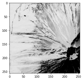
Here is the reversed image of black and white to make it easier to look at the snow condition

#Reversed image of black and white reversed image of black and white
img_nega = 255 - img_gray
io.imshow(img_nega)

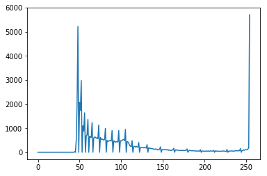
Confirmation of statistical information of the grayscaled data

Confirm the distribution in a histogram to estimate snow location.

print('pixel sum', np.sum(img_gray[:, :]))
print('pixel mean', np.mean(img_gray[:,:]))
print('pixel variance', np.var(img_gray[:,:]))
print('pixel stddev', np.std(img_gray[:,:]))
pixel sum 5346313
pixel mean 81.5782623291
pixel variance 5034.10730885
pixel stddev 70.9514433176

Confirmation of the histogram

hists, bins = np.histogram(img_gray, 255, [0, 255])
plt.plot(hists)

The following is the output.

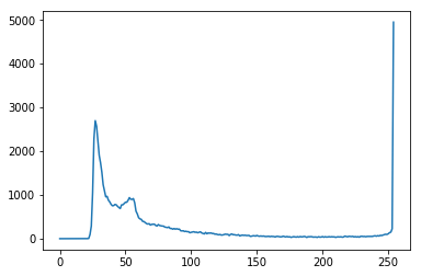
There are three obvious peak points: around 25, 55, and 250. The range 25-55 can be presumed as forests and rocks because it is relatively dark, and the range 250-255 as snow because it is almost white. Please note that, in this analysis, we can consider it as snow because it is visually confirmed that there was no cloud; however extra consideration will be required if conducted in cloudy conditions.

Extraction of the snowish part by determining the threshold

Binarize the grayscale image with a threshold value of 200, which is assumed to be the deepest location in the valley.

The procedure is as follows.

# Set the threshold
height, width= img_gray.shape
img_binary_gs200 = np.zeros((height, width)) # Initialize 
img_binary_gs200 = img_gray > 200 # Binarize based on threshold

io.imshow(np.concatenate(
   (color.gray2rgb(img_binary_gs200*255), img_true), axis=1))

Here is the calculated result.

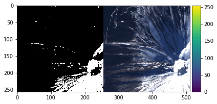
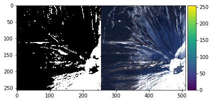
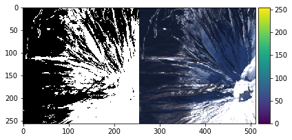
Although the brightest parts were extracted, snow in shaded areas completely failed. Change the threshold value to 80 and binarize the image again.

img_binary_gs80 = np.zeros((height, width)) # Initialize
img_binary_gs80 = img_gray > 80 # Binarize based on threshold

io.imshow(np.concatenate(
   (color.gray2rgb(img_binary_gs80*255), img_true), axis=1))

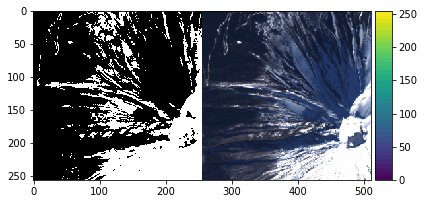
Although it seems snowy parts have been extracted relatively well, the upper right has not been extracted yet, so binarize the image again with the threshold value of 40.

img_binary_gs40 = np.zeros((height, width)) # Initialize
img_binary_gs40 = img_gray > 40 # Binarize based on threshold

io.imshow(np.concatenate(
   (color.gray2rgb(img_binary_gs40*255), img_true), axis=1))

Out[15]:

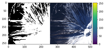
The range seems too broad this time.

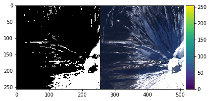
You can also use the Filter plug-in to set the threshold automatically to binarize the image, which is especially useful when such threshold value adjustment is needed.

th = filters.threshold_otsu(img_gray) # Determine threshold automatically
img_binary_gsauto = np.zeros((height, width))
img_binary_gsauto = img_gray > th

print("Threshold：", th)
io.imshow(np.concatenate(
   (color.gray2rgb(img_binary_gsauto*255), img_true), axis=1))
Threshold： 138



Out[16]:

Determination of snow conditions using HSV images

The snowish parts were roughly extracted; however, it shows the difficulty in setting the threshold value.

So let’s try a method other than grayscaling for detecting snow. We are going to use an image converted to HSV color space (Hue, Saturation, Value) to estimate the level of snow.

# Convert RGB to HSV
img_hsv = color.rgb2hsv(img_true)
io.imshow(img_hsv)

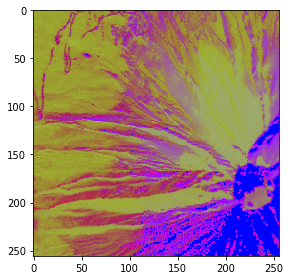
Confirmation of each component of HSV (Hue, Saturation, Value)

Check hue, saturation, and value respectively to confirm which component is related to snow.

im_conb_hsv = np.concatenate(( img_hsv[:, :, 0],  img_hsv[:, :, 1], img_hsv[:,:,2]), axis=1)
io.imshow(im_conb_hsv)

Now we are going to focus on the (component) value. Check the distribution of the value on the histogram.

hists, bins=np.histogram(img_hsv[:,:,2]*255, 255, [0, 255])
plt.plot(hists)

The cycle attributed to the use of color.rgb2hsv is observed. Dividing the peak value, set the threshold value at 150 and then look at the binarized image.

img_v = img_hsv[:,:,2]
# 閾値処理
height, width= img_v.shape
img_binary_v150 = np.zeros((height, width)) # 0で初期化
img_binary_v150 = img_v > 150 / 255 # 閾値にもとづいて2値化
​
io.imshow(np.concatenate(
   (color.gray2rgb(img_binary_v150*255), img_true), axis=1))



Out[20]:

To have the threshold value on the left side at peak value of 100, set the threshold value at 90 and binarize the image again.

img_v = img_hsv[:,:,2]
# Set the threshold
height, width= img_v.shape
img_binary_v90 = np.zeros((height, width)) # Initialize
img_binary_v90 = img_v > 90 / 255 #  Binarize based on threshold

io.imshow(np.concatenate(
   (color.gray2rgb(img_binary_v90*255), img_true), axis=1))

Comparison between RGB grayscaling and value methods

We tried estimating snow location with two different methods. Now compare the results achieved with each method.

io.imshow(np.concatenate(
   (color.gray2rgb(img_binary_gs80*255),
    color.gray2rgb(img_binary_v90*255),
    img_true), axis=1))

Out[22]:

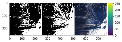
Comparing with the glayscaling method, the value method was better at determining snow including areas with shadows. It is important to consider shadowed areas when you have a bumpy mountain.

Though there exist other possible methods, we will finish here today.

(6) Summary

This article is one of the three-part series on the analysis using Tellus (snow condition analysis version)

The first part of the series covered logging in to Jupyter Notebook and extraction of the snow area.

The accuracy of the data is not guaranteed as this attempt was not based on scientific knowledge or theory. But this image analysis experiment has successfully illustrated the possibility of good snow condition analysis.

SORABATAKE will continue to conduct various experiments and verifications using Tellus. We would like to challenge interesting topics in a proactive way, so please let us know if you have any requests.

We also recommend you to try using Tellus to get some data in a wide range of topics. We only focused on visible lights in this article but will deal with SAR and other means in the next article.

We will use the snow index called NDSI (Normalized Difference Snow Index), which is used to estimate the ratio of snow cover to classify the snow condition in the next article.

Is it going to clearly explain snow conditions compared to the index used in this article? Don’t miss it!