[How to Use Tellus from Scratch] Get Himawari-8 Image and create animation using Jupyter Lab
We will explain how to get Himawari-8 image, and creating animation using Jupyter Lab on Tellus.
In this article, we will explain how to get Himawari-8 image, and to create its animation using Jupyter Lab on Tellus.
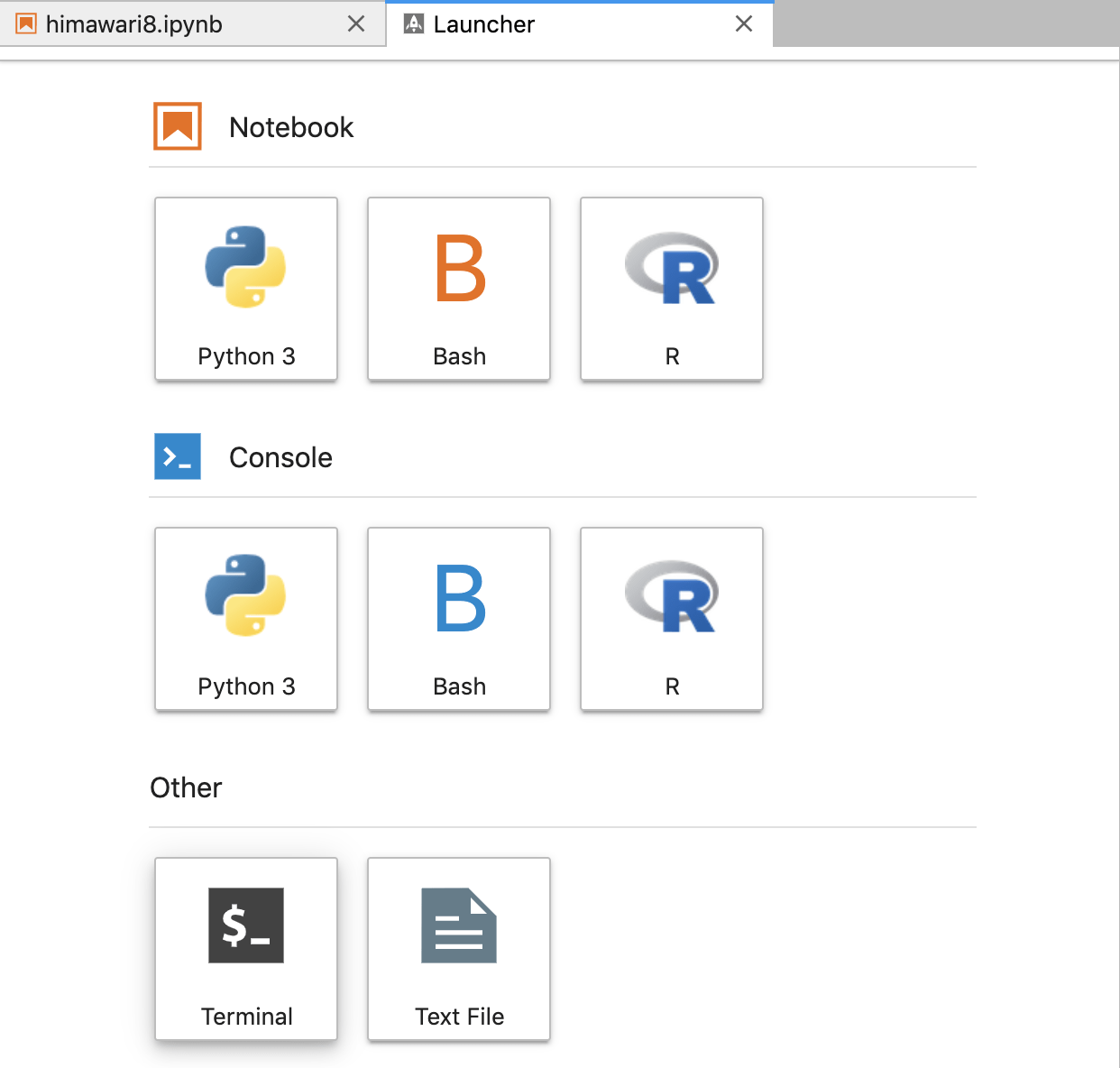
Please refer to “API available in the developing environment of Tellus” on how to use Jupyter Lab (Jupyter Notebook) on Tellus.
1. How to get Himawari-8 image
With Tellus API, you get image in monochrome from Himawari-8 (an optical band and four infrared bands).
For how to use API, a summary in the reference.
API reference
*Please make sure to check the data policy on Data Details as not to violate the terms and conditions when using images.
https://gsiapi.tellusxdp.com/api/v1/himawari8/{band}/{yyyy}/{mm}/{dd}/{hhmmss}/{z}/{x}/{y}.png| band | Bands to be acquired (B03/B07/B08/B13/B15 ) e.g.: B03 |
| yyyy | Acquisition year (western calendar, UTC) (2016/2017) e.g.: 2017 |
| mm | Acquisition month (double figures, UTC) e.g.: 04 |
| dd | Acquisition date (double figures, UTC) e.g.: 01 |
| hhmmss | Acquisition time (six figures, UTC) |
| Select 20 or 50 minutes of each hour e.g.: 005000 |
|
| z | Zoom level of the tile (1-4) only B03 corresponds up to 6 e.g.: 4 |
| x | X coordinate on the tile e.g.: 13 |
| y | Y coordinate on the tile e.g.: 6 |
*The available period for acquisition is from 00:50 (UTC) on January 1, 2016, to 23:50 (UTC) on December 31, 2017.
import requests
from skimage import io
from io import BytesIO
%matplotlib inline
TOKEN = ‘ここには自分のアカウントのトークンを貼り付ける’
def get_himawari8_scene(band, yyyy, mm, dd, hhmmss, z, x, y):
url = 'https://gisapi.tellusxdp.com/himawari8/{}/{}/{}/{}/{}/{}/{}/{}.png'.format(band, yyyy, mm, dd, hhmmss, z, x, y)
headers = {
'Authorization': 'Bearer ' + TOKEN
}
r = requests.get(url, headers=headers)
if r.status_code is not 200:
raise ValueError('status error({}).'.format(r.status_code))
return io.imread(BytesIO(r.content))
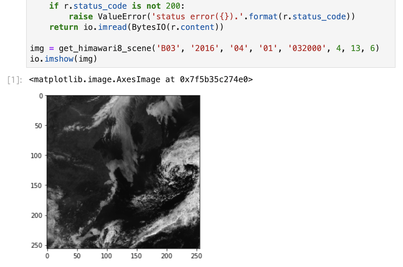
img = get_himawari8_scene('B03', '2016', '04', '01', '032000', 4, 13, 6)
io.imshow(img)
Get the token from APIアクセス設定 (API access setting) in My Page (login required).
Execute the code, and the image will be displayed.
2. Individual band characteristics of Himawari
As of July 2019, Tellus offers observation data in the following bands (wavelength bands) for approximately two years from 2016 to 2017.
- Band 3(visible) :0.64 μm μm
- Band 7(Infrared 4):3.9 μm
- Band 8 ( Infrared 3):6.2 μm
- Band 13(Infrared 1):10.4 μm
- Band 15(Infrared 2):12.4 μm
2.1 Band 3 (Visible)
Band 3 is a wavelength band that the human eye recognizes as red. It can observe lands, oceans, and clouds. It reflects sunlight well, displayed in white (that is, clouds, snow, and ice).
The observation depends on sunlight, so images will become darker at night.

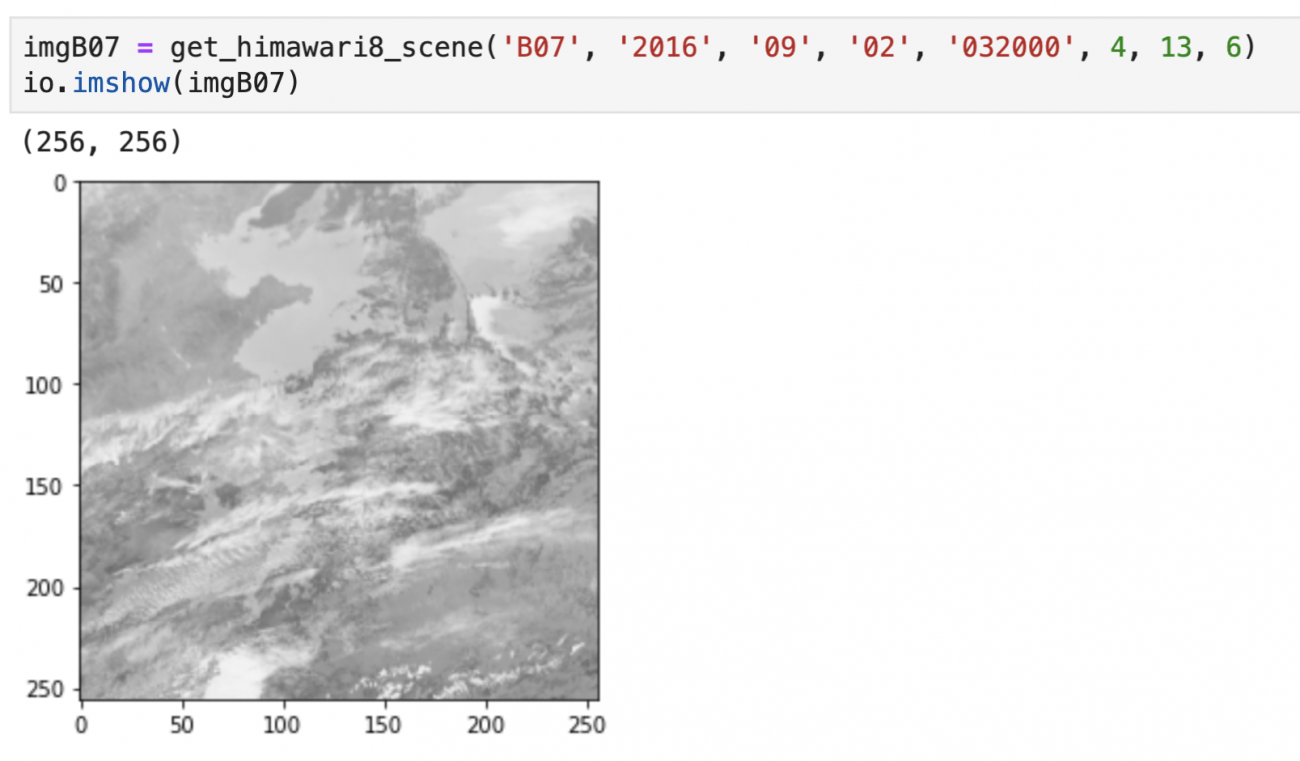
2.2 Band 7 (Infrared 4)
Band 7 is a wavelength band within the shortwave infrared region. It is a region of part sunlight and part black body radiation from the earth (electromagnetic waves emitted by a heated object). So a day image looks different from a night image.
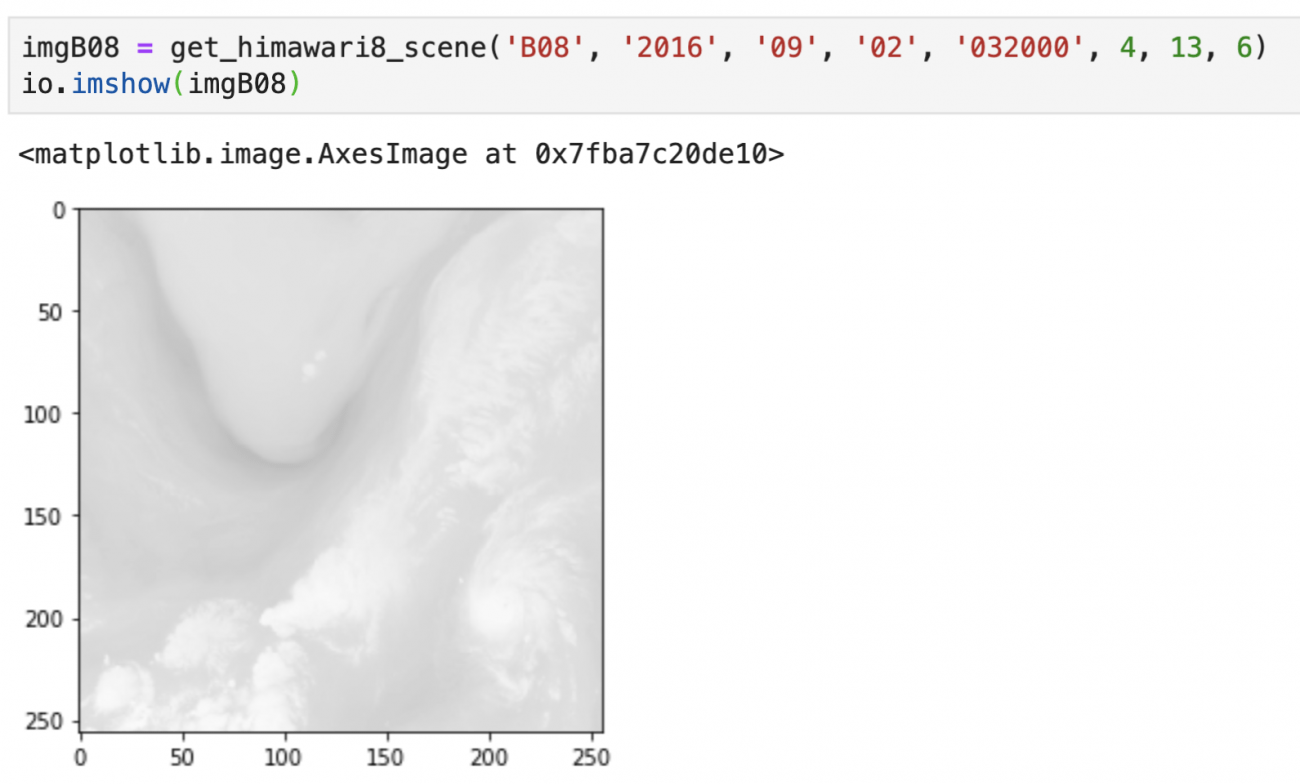
2.3 Band 8 (Infrared 3)
Band 8 is a wavelength band within a region called thermal infrared, having characteristics that are easily absorbed by water vapor.
With its characteristics, higher-altitude clouds are displayed whiter, and lower-altitude clouds darker.
2.4 Band 13 (Infrared 1)
Band 13 is a wavelength band within a region called thermal infrared. Unlike band 8, it is a wavelength that does not easily absorb water vapor.
Also, as it is not easily affected by sunlight, uniform observation is possible throughout the day and night.
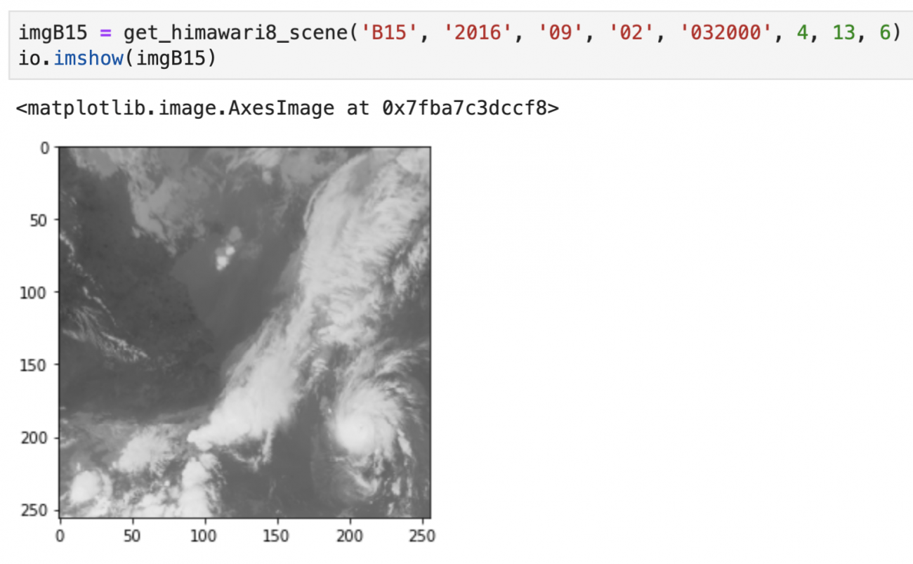
2.5 Band 15 (Infrared 2)
Band 15 is a wavelength band within a region called thermal infrared.
It has similar characteristics to band 13, but with band 15, the wavelength emitted by silicon hits maximum, (silicon is contained in volcanic ash or yellow sand), so it can mainly be used to observe atmospheric components. The human eyes can hardly distinguish between this and band 13.
3. Let's make cloud movements into animation
Finally, let’s create some animation using the Himawari image. This time, we would like to use Japanese text in the animation.
In the visualization library, with using (matplotlib), you cannot use Japanese in the default state, so please arrange fonts before moving the code.
To download Japanese fonts, execute the following command on the black screen opened from “Terminal.”
cd ~/work; wget https://ipafont.ipa.go.jp/old/ipafont/ipag00303.php; unzip ipag00303.php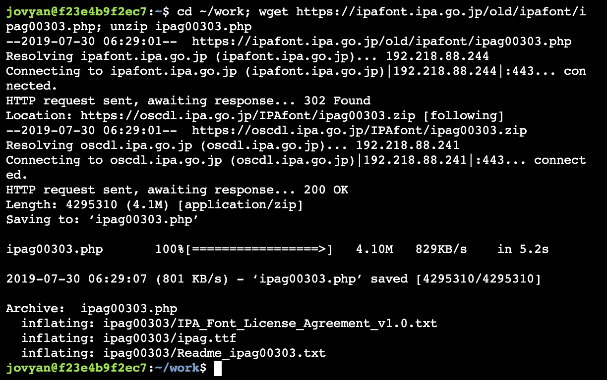
Now that Japanese fonts are ready, let’s create a sample code. In this sample, optical images for 72 hours from 9:00 on August 1, 2017, are combined to create a gif file.
import os
from pathlib import Path
from datetime import datetime
from datetime import timedelta
import matplotlib.pyplot as plt
import matplotlib.animation as animation
from matplotlib import font_manager as fm

basepath = Path(os.path.expanduser('~'))
fontpath = basepath / 'work/ipag00303/ipag.ttf' #フォントファイルの場所
font_prop = fm.FontProperties(fname=str(fontpath), size='large')
fig, ax = plt.subplots()

ims = []

begin_year = 2017
begin_month = 8
begin_day = 1
begin_hour = 9
hours = 72
interval_hours = 1
band = 'B03'
z = 4
x = 13
y = 6

begin_datetime = datetime(begin_year, begin_month, begin_day, begin_hour, 20, 0, 0) - timedelta(hours=9)
end_datetime = begin_datetime + timedelta(hours=hours)

temp_start = begin_datetime
while temp_start < end_datetime:
    try:
        title = ax.text(0.5, 1.05, 'ひまわり '+(temp_start + timedelta(hours=9)).strftime('%Y年%m月%d日%H時'),
                     ha='center', va='bottom', transform=ax.transAxes, fontproperties=font_prop) #日本語を使う箇所で毎回fontpropertiesを指定する

        img = get_himawari8_scene(band, str(temp_start.year), str(temp_start.month).zfill(2), str(temp_start.day).zfill(2), temp_start.strftime('%H%M%S'), z, x, y)

        ims.append([plt.imshow(img, cmap='gray'), title])

    except ValueError as e:
        print(e)
    temp_start = temp_start + timedelta(hours=interval_hours)

ani = animation.ArtistAnimation(fig, ims)

ani.save(str(basepath / 'work/himawari.gif'), writer=’pillow’)
plt.close()

from IPython.display import HTML
HTML('<img src="/work/himawari.gif">')
As the optical band (B03) images are combined, there will be regular time periods when nothing is shown.
Observation in the infrared band enables us to see during the night. If you are interested, try to create an infrared band animation by improving the sample code. Then, try to create an animation for different time periods or a place.
4. If your gif does not loop
You need to update your version of matplotlib.
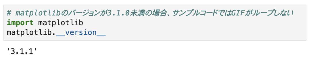
# matplotlibのバージョンが3.1.0未満の場合、サンプルコードではGIFがループしない
import matplotlib
matplotlib.__version__
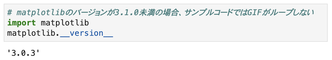
If the matplotlib version is less than 3.1.0, execute the update command ‘conda update matplotlib -y’ on the black screen (Terminal).
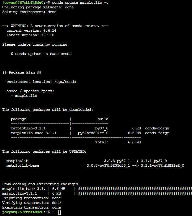
After the update, “Restart” Notebook on Lab, and try to move the sample code again.

It is successful if version notation is changed.
This time, we explain how to get Himawari-8 image and how to create an animation from an image using Jupyter Lab on Tellus.
The animation is applicable to other satellite images. Let’s improve not only the analysis but also data visualization.
References
Meteorological Satellite Center: Observation Image Characteristics