[How to Use Tellus from Scratch] Create an Elevation Graph of Mt. Fuji using Jupyter Lab
ASTER GDEM is a Digital Elevation Model (DEM) created based on the observational data of the optical sensor "ASTER" on NASA's Earth Observation Satellite, Terra. In this article, we will introduce how to create an elevation graph of Mt. Fuji with Jupyter Lab on Tellus using ASTER GDEM 2 elevation data.
In this article, we will introduce how to create an elevation graph of Mt. Fuji with Jupyter Lab.
Please refer to “API available in the developing environment of Tellus” for how to use Jupyter Lab (Jupyter Notebook) on Tellus.
1. Obtain an elevation data (ASTER GDEM 2)
Elevation data “ASTER GDEM 2” is available on Tellus.
ASTER GDEM is a Digital Elevation Model (DEM) created based on the observational data of the optical sensor “ASTER” on NASA’s Earth Observation Satellite, Terra.
ASTER GDEM 2 is its 2nd version, and it can obtain the elevation of the entire Earth with the resolution of 1 arc second in Latitude and Longitude (approximately 30m) and 1m in height direction.
*Elevation is a numerical value including the height of buildings and trees. Some parts do not include the height of buildings and trees.
The data can be obtained in the form of elevation tile using API. The elevation tile is a format to represent elevation data as a PNG image using the same coordinate as the map tile. The latitude and longitude of each pixel are represented by the value in the upper left and the elevation can be calculated from the RGB value.
Reference: Detailed specification of elevation tile
For how to use an API, it is summarized in this API reference.
*Please make sure to check the data policy on Data Details not to violate the terms and conditions when using data.
https://gisapi.tellusxdp.com/astergdem2/dsm/{z}/{x}/{y}.png引数
| z | Required | Zoom Level 0-12 |
| x | Required | X coordinate on the tile |
| y | Required | Y coordinate on the tile |
Let’s call up this API from Notebook on Jupyter Lab.
Open Tellus IDE, go to the “work” directory, select “Python 3,” and paste the following code.
import requests, json
from skimage import io
from io import BytesIO
%matplotlib inline

TOKEN = 'ここには自分のアカウントのトークンを貼り付ける'

def get_astergdem2_dsm(zoom, xtile, ytile):
    """
    ASTER GDEM2 の標高タイルを取得

    Parameters
    ----------
    zoom : str
        ズーム率
    xtile : str
        座標X
    ytile : number
        座標Y
    Returns
    -------
    img_array : ndarray
        標高タイル(PNG)
    """
    url = " https://gisapi.tellusxdp.com/astergdem2/dsm/{}/{}/{}.png".format(zoom, xtile, ytile)
    headers = {
        "Authorization": "Bearer " + TOKEN
    }

    r = requests.get(url, headers=headers)
    return io.imread(BytesIO(r.content))

img_12_3626_1617 = get_astergdem2_dsm(12, 3626, 1617)
io.imshow(img_12_3626_1617)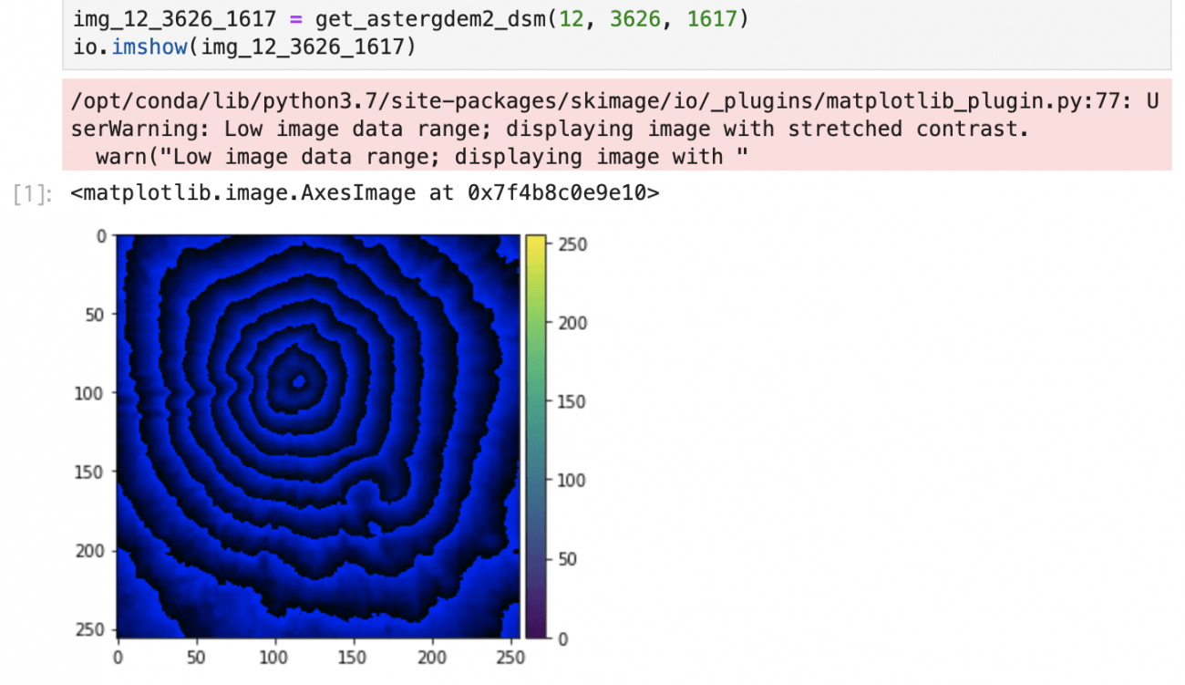
The elevation tile around the summit of Mt. Fuji is obtained in the sample code (z=12, x=3626, y=161) , (there may be a red warning, but it should not be a problem).
2. Calculate the elevation of Mt. Fuji
The elevation can be obtained from the RGB value of each pixel.
d = 65536 * R + 256 * G + B
When d < 8388608, h = d * u, when d = 8388608, h = NA, when d > 8388608, h = (d – 16777216)u.
Where u = 1.0.
In the elevation tile, the sea (elevation of 0 m) is indicated in black (R=0, G=0, B=0). Also, a point that could not be observed sufficiently is regarded as an error, and it is indicated in red (R=128, G=0, B=0).
Let’s create an elevation graph of Mt. Fuji using this formula. Scan the sequence equivalent to 138.73 degrees east longitude of the tile, z=12, x=3626, y=1617, in the latitude direction.
import math
import matplotlib.pyplot as plt

def get_tile_bbox(zoom, topleft_x, topleft_y, size_x=1, size_y=1):
    """
    タイル座標からバウンダリボックスを取得
    https://tools.ietf.org/html/rfc7946#section-5
    """
    def num2deg(xtile, ytile, zoom):
        # https://wiki.openstreetmap.org/wiki/Slippy_map_tilenames#Python
        n = 2.0 ** zoom
        lon_deg = xtile / n * 360.0 - 180.0
        lat_rad = math.atan(math.sinh(math.pi * (1 - 2 * ytile / n)))
        lat_deg = math.degrees(lat_rad)
        return (lon_deg, lat_deg)

    right_top = num2deg(topleft_x + size_x , topleft_y, zoom)
    left_bottom = num2deg(topleft_x, topleft_y + size_y, zoom)
    return (left_bottom[0], left_bottom[1], right_top[0], right_top[1])

def calc_height_chiriin_style(R, G, B, u=100):
    """
    標高タイルのRGB値から標高を計算する
    """
    hyoko = int(R*256*256 + G * 256 + B)
    if hyoko == 8388608:
        raise ValueError('N/A')
    if hyoko > 8388608:
        hyoko = (hyoko - 16777216)/u
    if hyoko < 8388608:
        hyoko = hyoko/u
    return hyoko

def plot_height(tile, index, direction, z, x, y, xtile_size=1, ytile_size=1, u=1):
    """
    高度のグラフをプロットする

    Parameters
    ----------
    tile : ndarray
        標高タイル
    bbox : object
        標高タイルのバウンディングボックス
    index : number
        走査するピクセルのインデックス
    direction : number
        走査方向(0で上から下、1で左から右)
    zoom : number
        ズーム率
    xtile : number
        座標X
    ytile : number
        座標Y
    xtile_size : number
        X方向のタイル数
    ytile_size : number
        Y方向のタイル数
    u : number
        標高分解能[m](デフォルト 1.0[m])
    """
    bbox = get_tile_bbox(z, x, y, xtile_size, ytile_size)
    width = abs(bbox[2] - bbox[0])
    height = abs(bbox[3] - bbox[1])
    if direction == 0:
        line = tile[:,index]
        per_deg = -1 * height/tile.shape[0]
        fixed_deg = width/tile.shape[1] * index + bbox[0]
        deg = bbox[3]
        title = 'height at {} degrees longitude'.format(fixed_deg)
    else:
        line = tile[index,:]
        per_deg = width/tile.shape[1]
        fixed_deg = -1 * height/tile.shape[0] * index + bbox[3]
        deg = bbox[0]
        title = 'height at {} degrees latitude'.format(fixed_deg)

    heights = []
    heights_err = []
    degrees = []
    for k in range(len(line)):
        R = line[k,0]
        G = line[k,1]
        B = line[k,2]
        try:
            heights.append(calc_height_chiriin_style(R, G, B, u))
        except ValueError as e:
            heights.append(0)
            heights_err.append((i,j))
        degrees.append(deg)
        deg += per_deg

    fig, ax= plt.subplots(figsize=(8, 4))
    plt.plot(degrees, heights)
    plt.title(title)
    ax.text(0.01, 0.95, 'Errors: {}'.format(len(heights_err)), transform=ax.transAxes)
    plt.show()

plot_height(img_12_3626_1617, 115, 0, 12, 3626, 1617)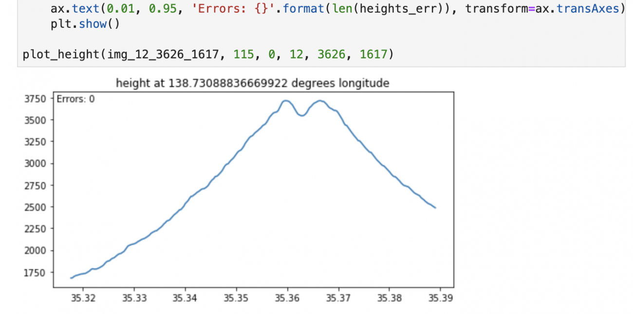
3. Calculate the elevation variability in Setagaya
Besides creating graphs, let’s play with the elevation data.
In the previous article “Made a hypothesis of a town where electric-assisted bicycles can be sold well with QGIS and actually visited the town”, Sorabatake searched for a town where electric-assisted bicycles can be sold well from satellite data.
In the article, we calculated the elevation variability among Tokyo’s 23 wards with QGIS, but is it possible to do the same thing with the data on Jupyter Lab and ASTER GDEM 2?
This time, we will try to calculate the elevation variability in Setagaya.
For the landform of each ward, we will use the administrative district data on National Land Numerical Information download services. Please refer to this article for how to download GeoJSON of the administrative district data.
In this article, we made the “data” directory under the “work” directory and uploaded GeoJSON there.
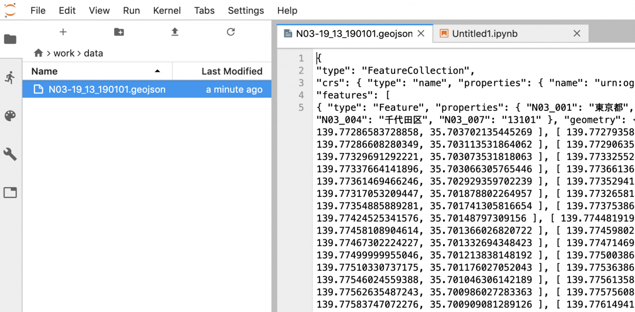
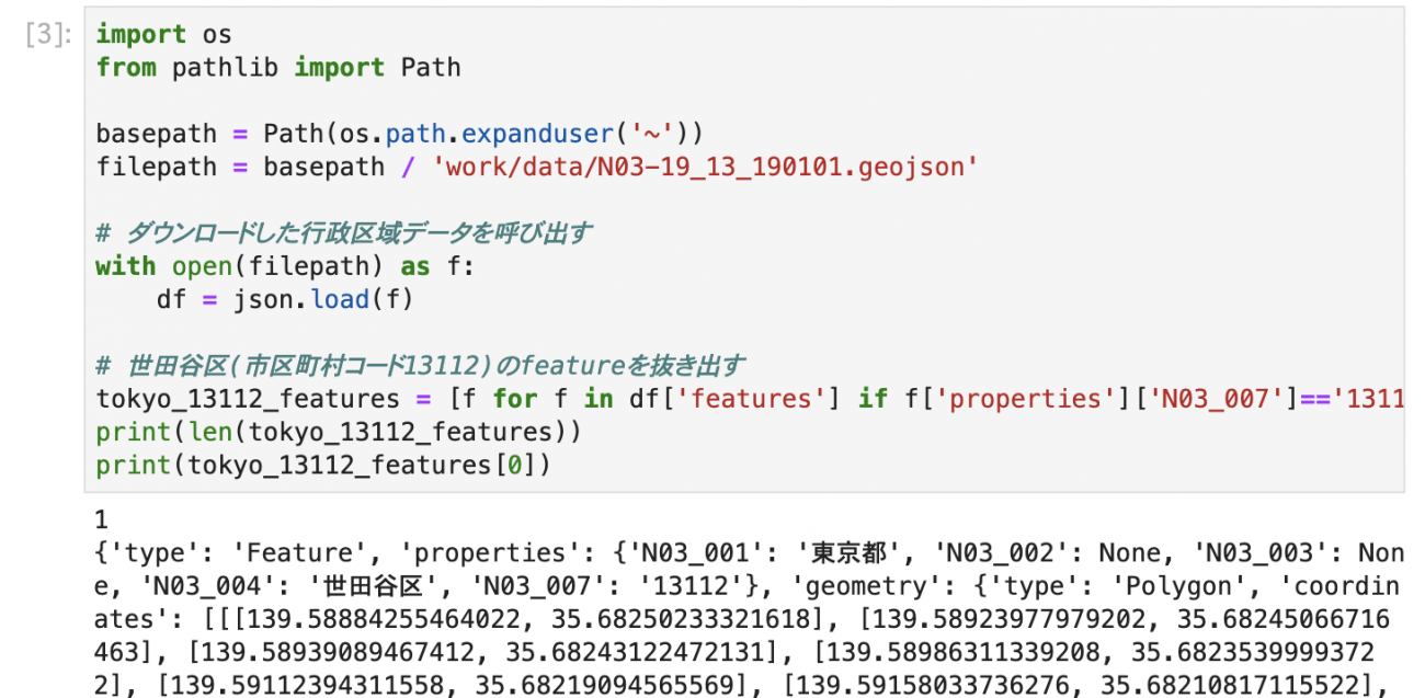
Load this GeoJSON, and extract the elements of the local government code 13112.
import os
from pathlib import Path

basepath = Path(os.path.expanduser('~'))
filepath = basepath / 'work/data/N03-19_13_190101.geojson'

# ダウンロードした行政区域データを呼び出す
with open(filepath) as f:
    df = json.load(f)

# 世田谷区(市区町村コード13112)のfeatureを抜き出す
tokyo_13112_features = [f for f in df['features'] if f['properties']['N03_007']=='13112']
print(len(tokyo_13112_features))
print(tokyo_13112_features[0])
Then, obtain the elevation tile that covers the entire Setagaya. At zoom level 12, connect six tiles in total, three vertically and two horizontally.
import numpy as np

def get_connected_astergdem2_dsm(zoom, topleft_x, topleft_y, size_x=1, size_y=1):
    """
    ASTER GDEM2 の標高タイルを size_x * size_y 分つなげた1枚の画像を作る
    """
    img = []
    for y in range(size_y):
        row = []
        for x in range(size_x):
            row.append(get_astergdem2_dsm(zoom, topleft_x + x, topleft_y + y))
        img.append(np.hstack(row))
    return  np.vstack(img)

tokyo_13112_img = get_connected_astergdem2_dsm(12, 3636, 1612, 2, 3)
io.imshow(tokyo_13112_img)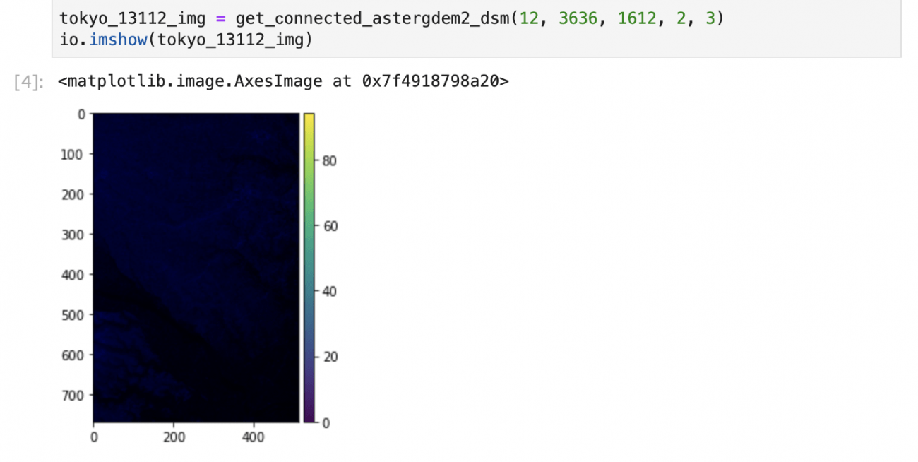
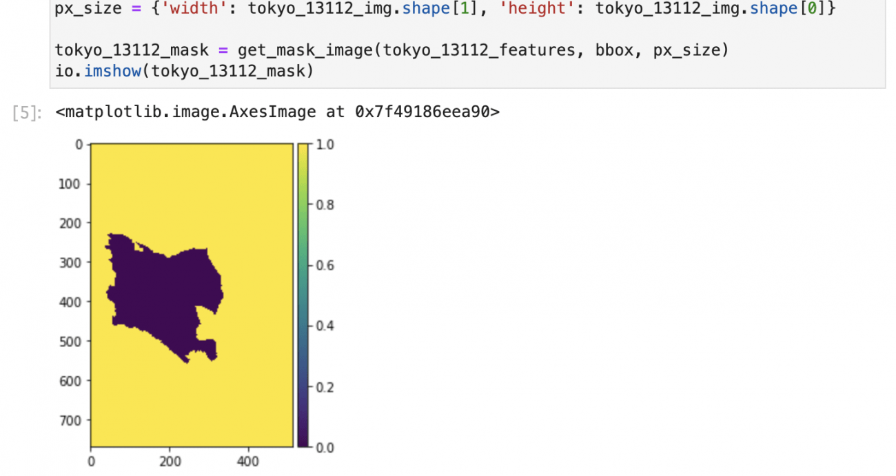
Next, create an image from the polygons of Setagaya, and create elevation tiles cut into the landform of Setagaya by overlaying them.
from skimage.draw import polygon

def get_polygon_image(points, bbox, img_size):
    """
    bboxの領域内にpointsの形状を描画した画像を作成する
    """
    def lonlat2pixel(bbox, size, lon, lat):
        """
        経度緯度をピクセル座標に変換
        """
        dist = ((bbox[2] - bbox[0])/size[0], (bbox[3] - bbox[1])/size[1])
        pixel = (int((lon - bbox[0]) / dist[0]), int((bbox[3] - lat) / dist[1]))
        return pixel

    pixels = []
    for p in points:
        pixels.append(lonlat2pixel(bbox, (img_size['width'], img_size['height']), p[0], p[1]))
    pixels = np.array(pixels)

    poly = np.ones((img_size['height'], img_size['width']), dtype=np.uint8)
    rr, cc = polygon(pixels[:, 1], pixels[:, 0], poly.shape)
    poly[rr, cc] = 0
    return poly

def get_mask_image(features, bbox, px_size):
    """
    図形からマスク画像を作成する

    Parameters
    ----------
    features : array of GeoJSON feature object
        マスクするfeature objectの配列
    bbox : array
        描画領域のバウンディングボックス
    px_size : array
        描画領域のピクセルサイズ
    Returns
    -------
    img_array : ndarray
        マスク画像
    """
    ims = []
    for i in range(len(features)):
        points = features[i]['geometry']['coordinates'][0]
        ims.append(get_polygon_image(points, bbox, px_size))

    mask = np.where((ims[0] > 0), 0, 1)
    for i in range(1,len(ims)):
        mask += np.where((ims[i] > 0), 0, 1)

    return np.where((mask > 0), 0, 1).astype(np.uint8)

bbox = get_tile_bbox(12, 3636, 1612, 2, 3)
px_size = {'width': tokyo_13112_img.shape[1], 'height': tokyo_13112_img.shape[0]}

tokyo_13112_mask = get_mask_image(tokyo_13112_features, bbox, px_size)
io.imshow(tokyo_13112_mask)
def clip_image(img, mask):
    """
    図形をマスクする

    Parameters
    ----------
    img : ndarray
        加工される画像
    mask : ndarray
        マスク画像
    Returns
    -------
    img_array : ndarray
        マスクされた画像
    """
    base = img.transpose(2, 0, 1)[:3,:]
    cliped = np.choose(mask, (base, 0)).astype(np.uint8)
    return cliped.transpose(1, 2, 0)

tokyo_13112_cliped = clip_image(tokyo_13112_img, tokyo_13112_mask)
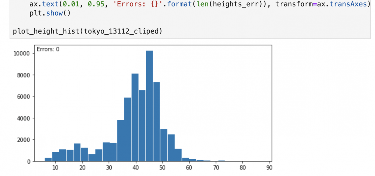
With the elevation tile cut into the landform of wards, let’s create a histogram of the height.
def get_height_array(tile, u):
    """
    標高タイルから高さの配列を作る
    ただしエラーや0メートル地点は配列から除く
    """
    heights = []
    heights_err = []
    for i in range(tile.shape[0]):
        for j in range(tile.shape[1]):
            R = tile[i, j, 0]
            G = tile[i, j, 1]
            B = tile[i, j, 2]
            try:
                heights.append(calc_height_chiriin_style(R, G, B, u))
            except ValueError as e:
                heights.append(0)
                heights_err.append((i,j))
    heights = np.array(heights)
    return (heights[heights > 0], heights_err)

def plot_height_hist(tile, u=1):
    """
    標高タイルから高さのヒストグラムを作る

    Parameters
    ----------
    tile : ndarray
        標高タイル
    """
    (heights, heights_err) = get_height_array(tile, u)

    fig, ax= plt.subplots(figsize=(8, 4))
    plt.hist(heights, bins=30, rwidth=0.95)
    ax.text(0.01, 0.95, 'Errors: {}'.format(len(heights_err)), transform=ax.transAxes)
    plt.show()

plot_height_hist(tokyo_13112_cliped)
Finally, obtain statistical information such as variance and mean.
def calc_height_statistics(tile, u=1):
    """
    標高タイルの高さの統計情報を求める

    Parameters
    ----------
    tile : ndarray
        標高タイル
    Returns
    -------
    result_object : object
        統計情報
    """
    (heights, heights_err) = get_height_array(tile, u)
    return {'std': np.std(heights), 'mean': np.mean(heights), 'max': np.max(heights), 'min': np.min(heights)}

print(calc_height_statistics(tokyo_13112_cliped))

Although the calculation method and the original data are different, roughly the same result could be obtained as the result of the previous article.The same procedure can be used for other wards.
This is how to create an elevation graph of Mt. Fuji using Jupyter Lab on Tellus. Although the data of ASTER GDEM 2 is less accurate than the elevation data provided by the Geospatial Information Authority of Japan, it is excellent as the data missing range is small and that it can cover locations outside the country. So please take advantage of it.