Representing Satellite Orbits with Python – Orbital Elements, TLE
Part 2 of the satellite orbits series! This time, we'll be using Python to represent the orbits of artificial satellites.
In this article, we will practically learn how to represent orbits using the method introduced in the previous article.
Preparation:
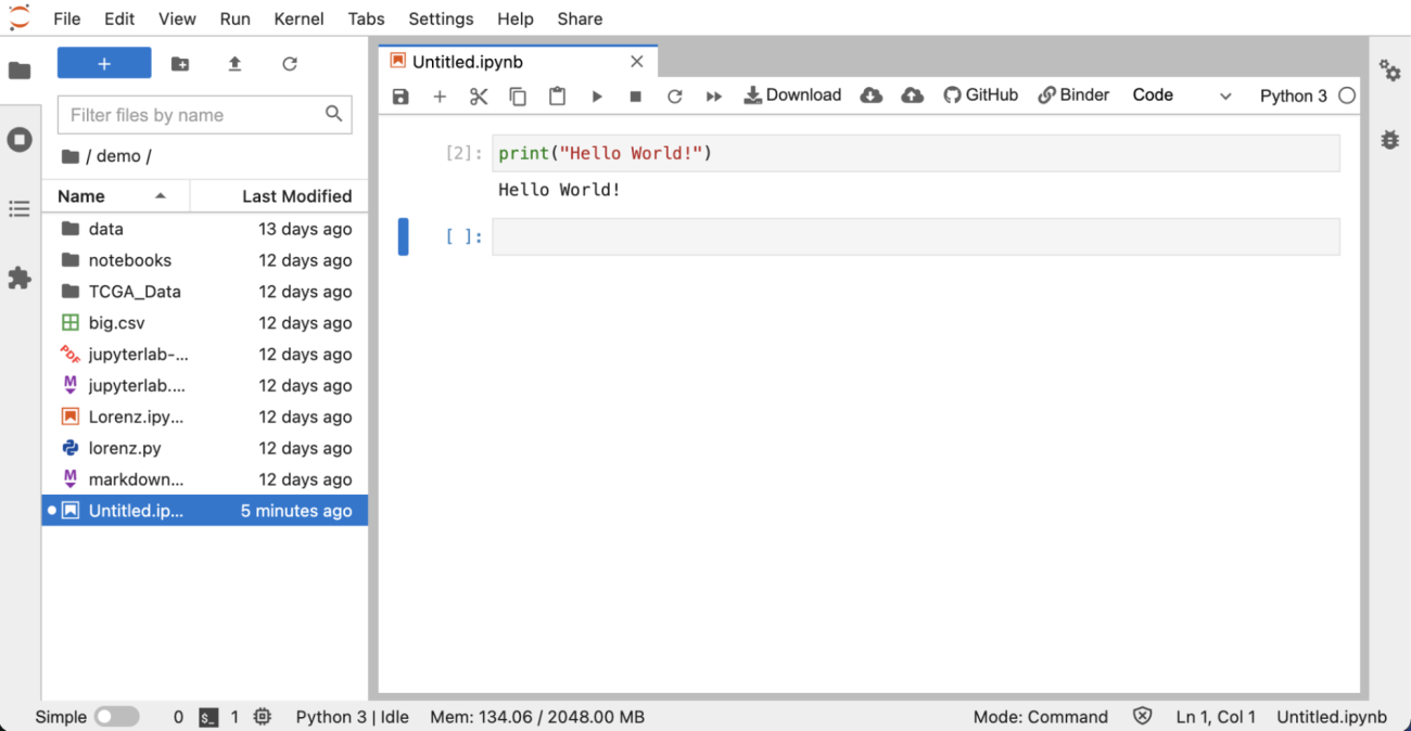
In this article, we will be using the Jupyter notebook from Try Jupyter to explain while performing actual calculations. First, go to the Try Jupyter URL (https://jupyter.org/try), select “Try JupyterLab,” click on [File] > [New Notebook] > [Python3] to open a Python notebook environment. In a notebook cell, type:
print("Hello World!")Then click [Run] (or select the cell and press Shift+Enter). If you see “Hello World!” displayed, you have successfully set up Try Jupyter.
Orbit Representation Methods:
Before explaining orbits as destinations, let’s first understand how satellites and spacecraft move in orbits.
When you throw a ball on the ground, it follows a parabolic path and eventually lands on the ground. The trajectory followed by this ball and the orbit of a satellite or spacecraft operate on exactly the same principle (although in reality, due to atmospheric resistance, objects on Earth undergo more complex motions than those in space).
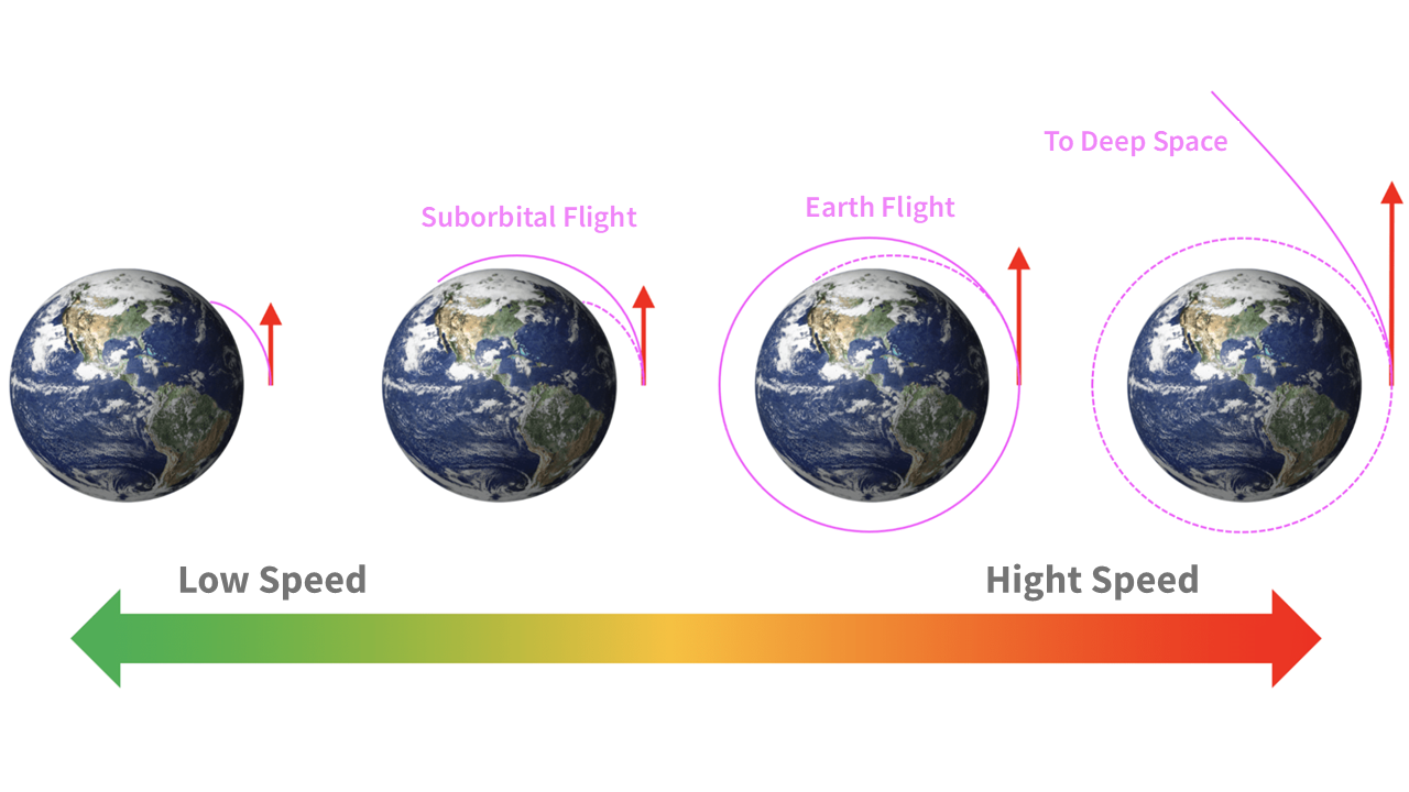
If you throw the ball faster, it will travel farther. While human physical capabilities have limits, with technology, humans can propel objects faster and farther. Eventually, we were able to reach outer space, surpassing altitudes of 100 kilometres.
Once in space, objects following a trajectory that brings them back to Earth are referred to as having a “suborbital” trajectory.
By further increasing speed, an object can remain in space indefinitely. This is known as an Earth orbit, and it’s the type of trajectory artificial satellites, often referred to as Earth-orbiting satellites, follow.
With even greater speed, a satellite can break free from Earth’s gravity and journey into deep space.
Newton's Second Law and Orbital Mechanics:
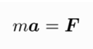
Let’s delve into a bit of theory (this section requires knowledge of calculus, vectors, etc., so feel free to skip if you’re not interested). Both a ball thrown on the ground and an artificial satellite flying in space follow Newton’s second law, as shown below:
↓
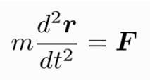
Where m represents mass of the probe, a is the acceleration of the vector, and F is the force acting on the probe, r denotes the position of the vector of the satellite.
For Earth-orbiting artificial satellites in particular, they move under the influence of Earth’s gravity. Using Newton’s law of universal gravitation, it can be expressed as:
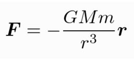
Here, G is the universal gravitational constant, M is the mass of the Earth, and m is the mass of the probe. r represents the distance from the centre of the Earth to the satellite, where the vector r signifies the position vector of the satellite from the centre of the earth.
By numerically solving this Newtonian equation of motion, we can calculate the orbit of an artificial satellite. Since this can be done with a short program, feel free to run the following code in Jupyter if you’re interested. Additionally, try changing the values of x0 and t to see how the orbit changes.
Furthermore, determining where an artificial satellite located at a certain position and velocity at a given time will be at a later time is referred to as “Orbit Propagation.” Experts like us engage in orbit propagation on a daily basis. For the case of a satellite orbiting a single celestial body, such as Earth, orbit calculation can be done analytically (with simple equations). However, for more complex orbit propagation, numerical calculations are required.
# Import Python Modules
import numpy as np # Numerical computation library
from scipy.integrate import odeint # Library for solving ordinary differential equations
import matplotlib.pyplot as plt # Plotting library

# Equations of motion for the two-body problem
def func(x, t):
    GM = 398600.4354360959 # Earth's gravitational constant, km^3/s^2
    r = np.linalg.norm(x[0:3])
    dxdt = [x[3],
            x[4],
            x[5],
            -GM*x[0]/(r**3),
            -GM*x[1]/(r**3),
            -GM*x[2]/(r**3)]
    return dxdt

# Initial conditions for the differential equations
x0 = [10000, 0, 0, 0, 7, 0] # Position (x,y,z) + Velocity (vx,vy,vz)
t  = np.linspace(0, 86400, 1000) # One day's worth of orbit propagation

# Numerical solution of the differential equations
sol = odeint(func, x0, t)

# Plotting
plt.plot(sol[:, 0],sol[:, 1], 'b')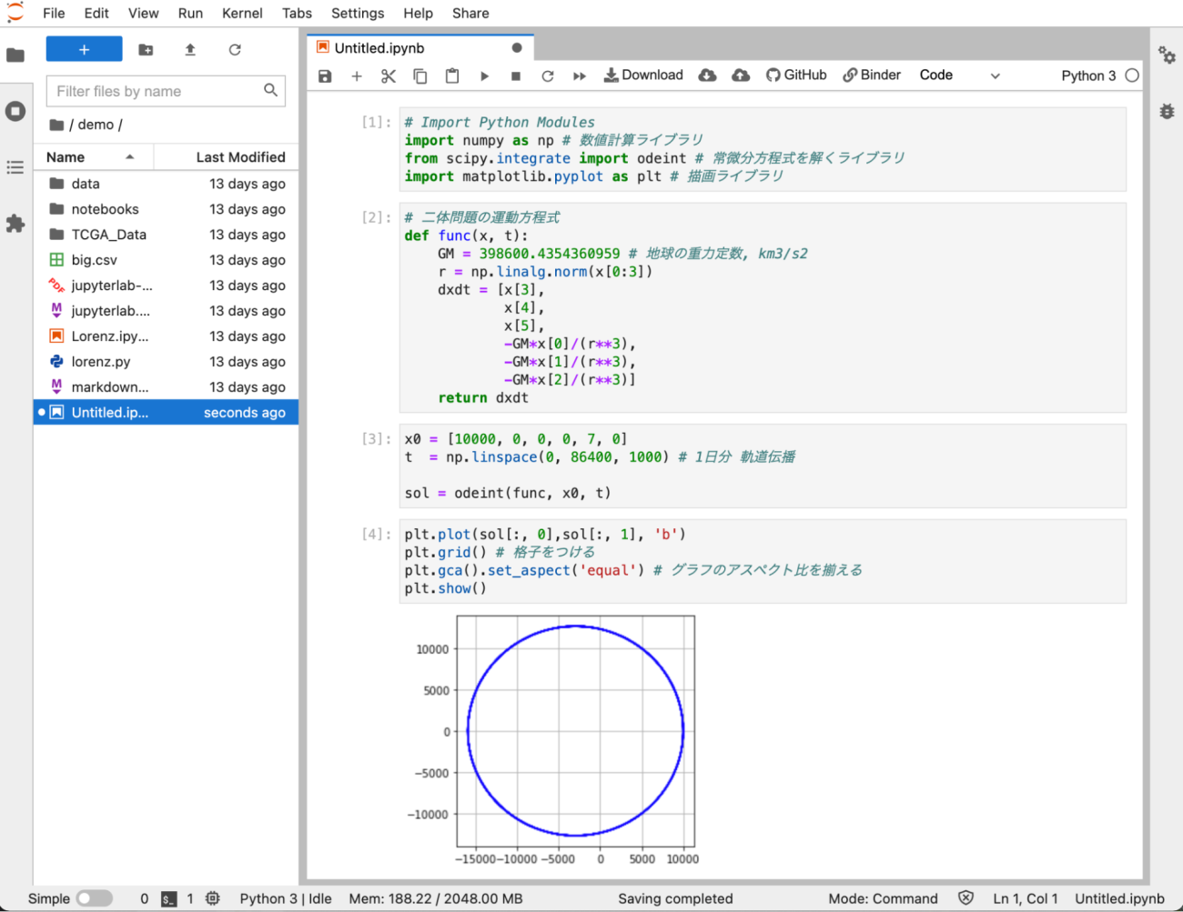
Orbital 6 elements:
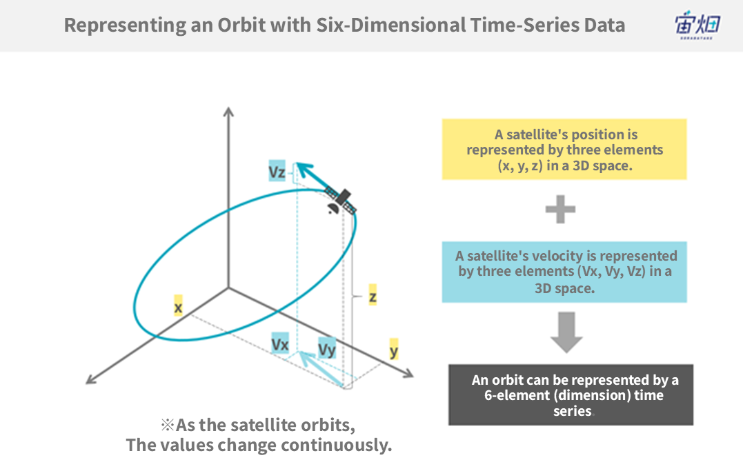
Planets and artificial satellites’ orbits can be represented by a time series of six dimensions, which includes three dimensions for position and three for velocity.
In particular, planets that are influenced solely by the gravity of the Sun move in an “elliptical orbit,” a discovery made by the astronomer Johannes Kepler.
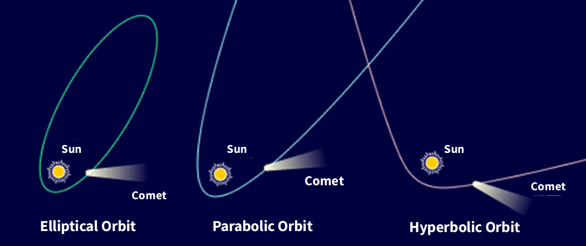
The behaviour of an object that moves under the influence of the gravity of a single celestial body, such as the Sun, is referred to as solving the “two-body problem.” It is known that an object moving under the two-body problem follows one of three types of orbits: “elliptical orbit,” “parabolic orbit,” or “hyperbolic orbit.”
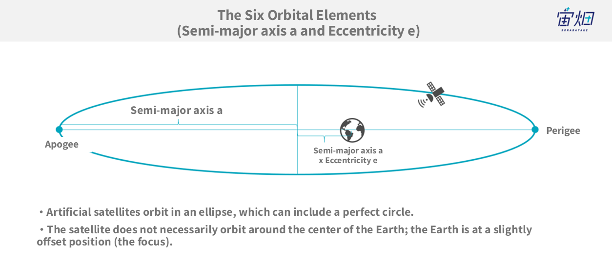
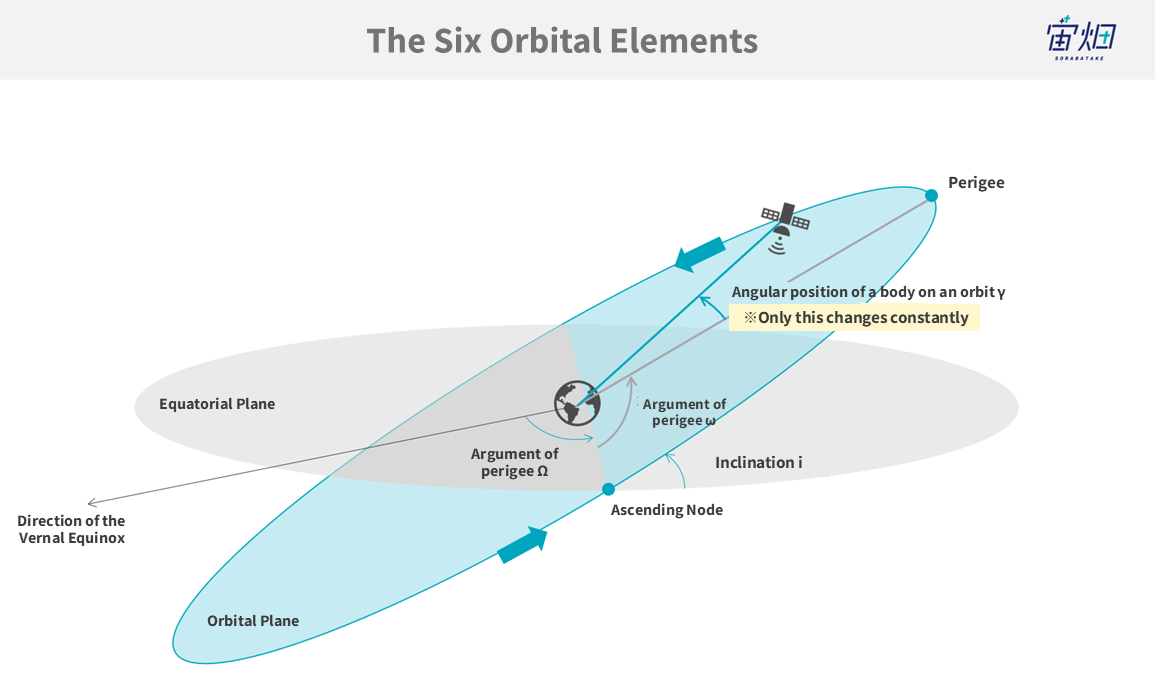
By utilising the property that orbits move according to the two-body problem, the orbits of planets and artificial satellites can be represented in a more manageable form. This is what we call the “orbital six elements.” There are various ways to determine the six orbital elements, but the most commonly used ones are as follows:
1.Semi-major axis (a)
2.Eccentricity (e)
3.Inclination (i)
4.Longitude of the ascending node (Ω)
5.Argument of perigee (ω)
6.True anomaly, eccentric anomaly, or mean anomaly (ν, E, or M)
We will omit the detailed explanation of each element here.
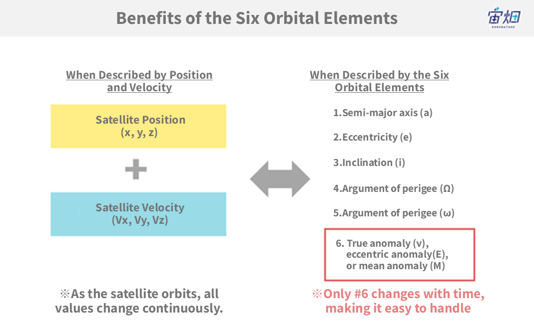
Now, why do we deliberately choose to represent them using the orbital six elements? This is because in the case of an object moving under the two-body problem, five of the elements (a, e, i, Ω, ω) do not change over time.
Of course, real-world artificial satellites, apart from being affected by Earth’s gravity, also experience forces due to the gravity of the Sun and the Moon, Earth’s atmospheric resistance, and the fact that Earth is not a perfect sphere. Thus, (a, e, i, Ω, ω) change constantly. Nonetheless, in many cases, using the orbital six elements, which vary only slightly, is theoretically more convenient.
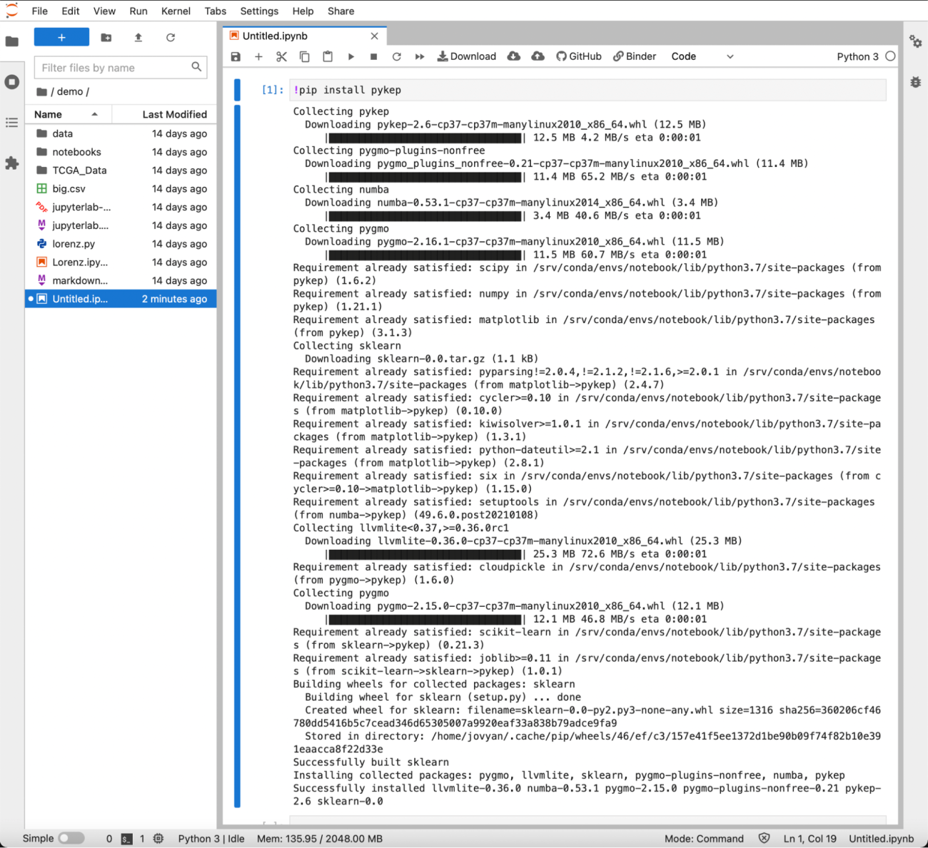
Now, let’s use a Jupyter Notebook to actually convert between the orbital six elements and position-velocity. For this calculation, we will use a library called pykep released by the Advanced Concepts Team (ACT) of the European Space Agency (ESA). First, install pykep in your Jupyter Notebook using the following command (installation will take a few tens of seconds):
!pip install pykepIf the screen shows something like below, the installation was successful:
The six orbital elements of Earth’s orbit (in heliocentric, ecliptic coordinates) are as follows (reference: https://ssd.jpl.nasa.gov/txt/aprx_pos_planets.pdf). For calculation with pykep, we’ll convert them to units of km and rad:
|
Six Elements of Earth’s Orbit
(Sun-centred, ecliptic plane reference coordinate system)
|
||
|
(au, deg)
|
(km, rad)
|
|
| Semi-major axis a: | 1.00000261 au | 149598261.1504 km |
| Eccentricity e: | 0.01671123 | 0.01671123 |
| Inclination i: | -0.00001531 deg | -2.6720990848033185e-07 rad |
| Longitude of ascending node Ω: | 0.0 deg | 0.0 rad |
| <span style="font-weight: 400;"Argument of perigee ω: | 102.93768193 deg | 1.796601474049171 rad |
| Eccentric anomaly E: | Calculated depending on the desired time | Calculated depending on the desired time |
We’ll use the function par2ic from pykep to convert the orbital six elements into position r
and velocity v. Note that we’ll use a value of 132712440041.9393 km³/s² for the solar gravitational constant, which is needed for the conversion. Be sure to import the module since it’s required to use the installed pykep module.
import pykep as pk
GM = 132712440041.9393 # km3/s2
r, v = pk.par2ic([
                    149598261.1504, # a, km
                    0.01671123, # e, -
                    -2.6720990848033185e-07, # i, rad
                    0.0, # O, rad
                    1.796601474049171, # w, rad
                    0.0 # E, rad
                 ], GM)
print(r, v)
You should see a value like this: (-32934004.25725372, 143364076.19608086, -38.308301679723) (-29.51776907469439, -6.780906055160861, 1.8119252864133049e-06). This represents the position and velocity of Earth when the eccentric anomaly E is 0 (when Earth is at its closest point to the Sun).
Conversely, if you’re given the position and velocity, you can use the module ic2par from pykep to obtain the six orbital elements.
Now, let’s vary the eccentric anomaly E for one orbit and display the result using a plotting library. This way, we’ve managed to draw the (almost) elliptical orbit of Earth.
import numpy as np
import matplotlib.pyplot as plt
import pykep as pk

GM = 132712440041.9393  # km3/s2
ea_all = np.linspace(0, 2*np.pi, 1000)  # 0 to 2pi radian

pos = np.array([
    pk.par2ic([
        149598261.1504,  # a, km
        0.01671123,  # e, -
        -2.6720990848033185e-07,  # i, rad
        0.0,  # O, rad
        1.796601474049171,  # w, rad
        ea_t  # E, rad
    ], GM)[0]  # Take only the position
    for ea_t in ea_all
])  # Calculate in bulk using a list comprehension

# Plotting
plt.plot(pos[:, 0], pos[:, 1], 'b')
plt.grid()
plt.gca().set_aspect('equal')
plt.show()
To calculate the position and velocity of planets like Earth, experts like us use libraries like SPICE(https://naif.jpl.nasa.gov/naif/toolkit.html) provided by NASA JPL, which utilize ephemerides (celestial histories). With ephemerides, you can calculate high-precision positions and velocities that take into account the influences of multiple celestial bodies’ gravities. There’s also a Python library called spiceypy (https://github.com/AndrewAnnex/SpiceyPy) provided for this purpose. If you’re interested, feel free to give it a try.
2-Line Orbital Element Set (TLE):
For Earth-orbiting satellites, particularly those in low orbits, a data format known as Two-Line Element Set (TLE) is sometimes used to represent their orbital information. TLE is a data format that encapsulates various Earth-centred orbital elements still utilised by organisations like NASA and the North American Aerospace Defense Command (NORAD).
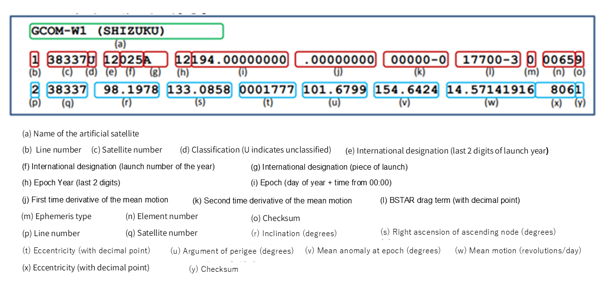
Explanation of Each TLE Element:
・Satellite Catalog Number (25544U)
・NORAD Catalog Number (98067A)
・Epoch Year (21226.49389238)
・First Time Derivative of the Mean Motion (0.00001429)
・Second Time Derivative of Mean Motion (00000-0)
・BSTAR drag term (34174-4)
・Element Set Number (0 9998)
For example, the TLE for the International Space Station (ISS) as of August 15, 2021, is as follows:
ISS (ZARYA)
1 25544U 98067A 21226.49389238 .00001429 00000-0 34174-4 0 9998
2 25544 51.6437 54.3833 0001250 307.1355 142.9078 15.48901431297630
The orbital information represented by TLE is often converted to position and velocity using algorithms like the Simplified General Perturbations Satellite Orbit Model 4 (SGP4). The SGP4 algorithm is provided as a Python library, allowing calculations to be performed in a Jupyter notebook.
To install the SGP4 library, execute the following command:
!pip install sgp4Next, let’s calculate the position and velocity of the ISS:
from sgp4.api import Satrec, jday

# TLE for the ISS
s = '1 25544U 98067A   21226.49389238  .00001429  00000-0  34174-4 0  9998'
t = '2 25544  51.6437  54.3833 0001250 307.1355 142.9078 15.48901431297630'

# Calculate position and velocity using SGP4
satellite = Satrec.twoline2rv(s, t)
jd, fr = jday(2021, 8, 15, 0, 0, 0)
e, r, v = satellite.sgp4(jd, fr)

# Output the results
print(r)  # True Equator Mean Equinox position (km)
print(v)  # True Equator Mean Equinox velocity (km/s)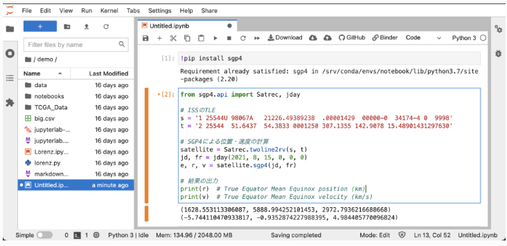
That’s it! This demonstrates how orbital information of satellites is represented using Python. In the next article, we’ll use the representation methods we’ve learned here to introduce commonly used types of orbits.