The conversion of SAR to optical image using pix2pix and analysis of another SAR image with this generator
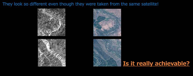
Using GANs, which has become a popular topic in recent years as an image generation algorithm, I tried to convert non-intuitive SAR images into optical images.
In this article, I try to convert SAR images into more user-friendly data using GANs, which have been getting a lot of attention recently as an image generation algorithm, I tried two different types of satellite data: optical images, which are easy to understand by the human eye; and SAR images, which are difficult to understand at a glance.
First, I will briefly explain the difference between optical and SAR images.
[Optical image]
The properties of an object measured at a distance are analyzed by measuring the scattered light against sunlight using light-based remote sensing technology (generally, the term “satellite image” is often used to refer to this type of image). However, it is not possible to observe areas covered by clouds or at night.
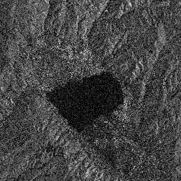
[SAR image]
The properties of an object measured at a distance are analyzed by observing the reflected waves when the object is irradiated with radio waves. Although a SAR image looks quite different from an optical image, it can be observed through clouds and at night. In addition, it is useful in times of disaster such as earthquakes because we can observe ground deformation and other phenomena using phase information.
As you can see, optical images are familiar because they basically show something similar to what you see in Google Earth.
*Since measurements are made using the lightwave range, it is also possible to conduct measurement by combining various wavelengths, including the near-infrared, which is invisible to the human eye.
On the other hand, SAR images measured in the radio range are completely different in appearance and characteristics from easy-to-understand optical images. As you can see from the image, SAR images are difficult for beginners to understand and handle.
If we can improve the readability of SAR images, the use of satellite images will become more widespread. In order to achieve this, it is important to understand the relationship between SAR images and optical images.
In addition, recent advances in satellite technology have made it possible to make detailed measurements using multiple sensors and parameters. However, in the past, there were many optical and SAR images that were observed with poor resolution or gray-scale images. And so, it is also an important challenge to gain more detail and important information from such limited data based on the past.
As an approach to the above-mentioned challenge, in this article, I analyze the relationship between the SAR image and the optical image by implementing a method to convert SAR images into optical images using machine learning.
As for the actual machine learning method, I trained pix2pix, a type of GANs, which are a well-known image generation algorithm, for the conversion from SAR images to optical images. We also trained pix2pix for the conversion from grayscale optical images to RGB optical images for comparison.
*The training was performed using the Sentinel-1 (SAR) and Sentinel-2 (optical image) pairs, which can be found outside of Tellus, because these implementations require a large number of data sets in which the topography of SAR and optical images are identical, and it would take a huge amount of time to create them individually.
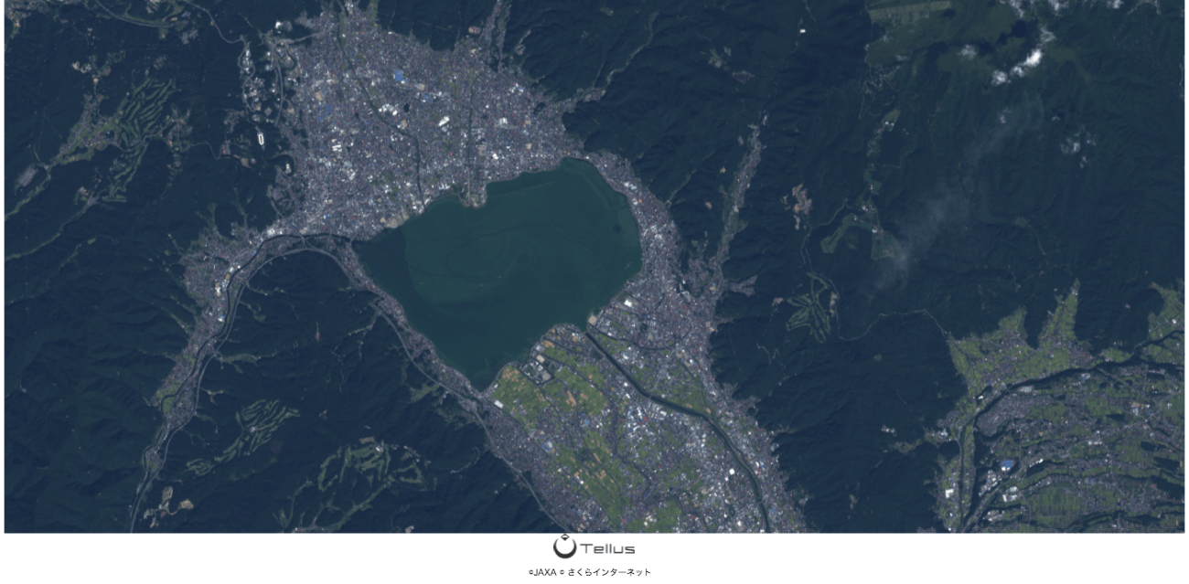
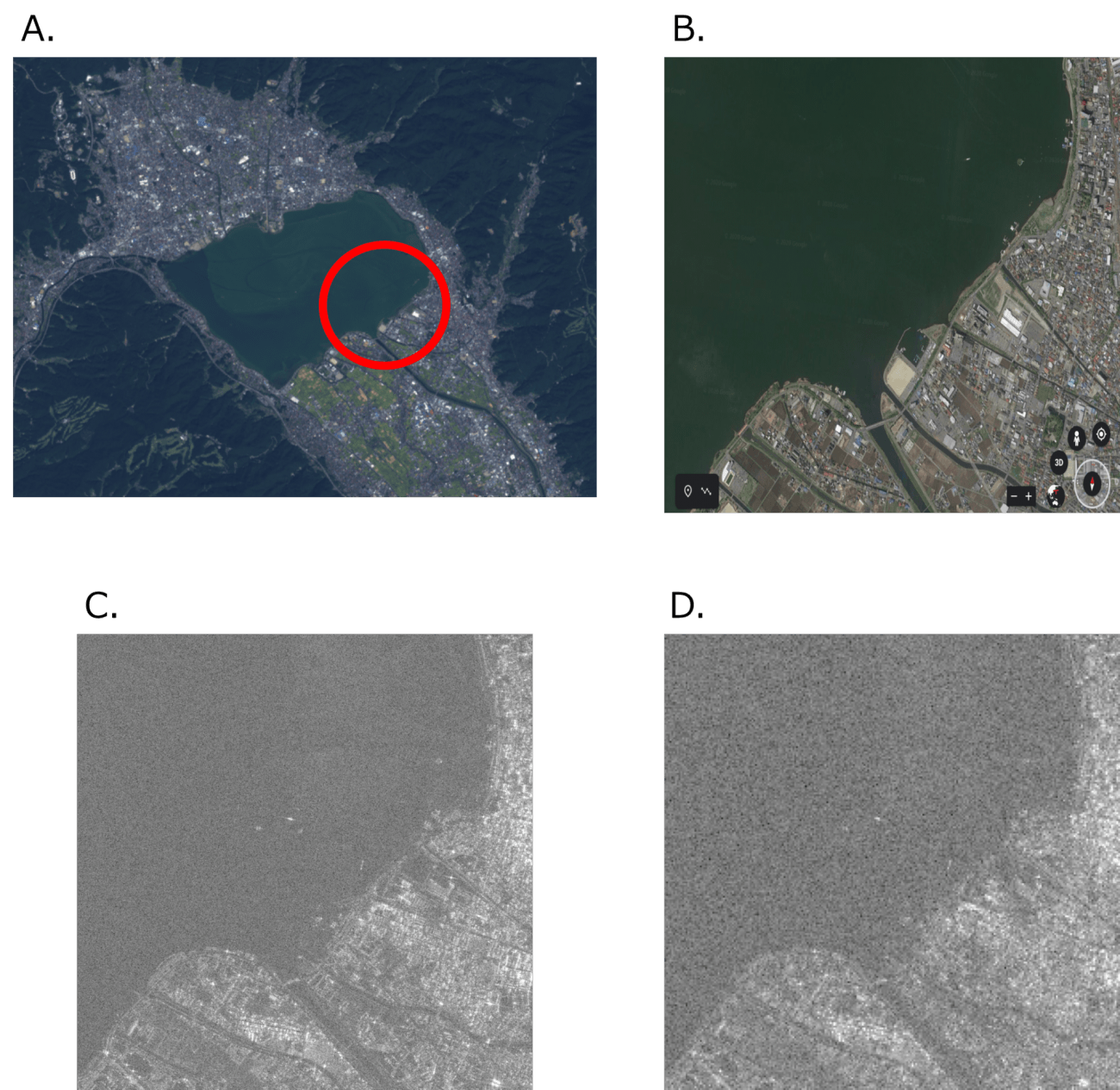
In addition, we would like to show you what kind of results we got when we tried to convert SAR images around Lake Suwa (Fig. 2) of PALSAR2 available on Tellus into color RGB images using the following two generators made by pix2pix: (1) generator for converting SAR image (grayscale) into optical image (RGB) and (2) generator for converting optical image (grayscale) into optical image (RGB).
(1) What are GANs (Generative Adversarial Networks)?
Now, before I introduce you to the actual results, let me explain the GANs, which are the crux of this challenge.
GANs are a technique with a structure that learns two networks (generator and discriminator) to compete with each other (pix2pix used for this challenge is one type of the GANs).
While the generator makes a real-like false image from the input image, the discriminator compares the false image made by the generator with the real image to determine which one is the real one. The generator tries to make the image look as real as possible, and the discriminator tries its best to judge the image made by the generator as a fake. The main characteristic of GANs is to find the regularities and features that make the acquired images look like the real ones through this competitive process.
Pix2pix, the technique used here, has the following features compared to the general GANs.
– Pix2pix uses the original image as input instead of random noise like general GANs.
– Pix2pix adds noise by introducing dropouts during learning and testing.
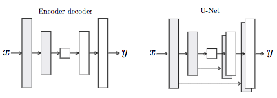
– Pix2pix combines the encoder information with the decoder of U-Net, an encoder-decoder, into a generator.
– L1 loss is introduced in the loss function of the generator, which prevents the image from being blurred. – Also, it becomes closer to the original image when the ratio of L1 loss is increased.
Roughly speaking, the generator of normal GANs makes false images in the following order: (1) Noise, (2) Extend dimension, (3) Reduce dimension, and (4) Generate image. The generator of pix2pix, on the other hand, makes false images in the following order: (1) Original image, (2) Extend dimension, (3) Reduce dimension, and (4) Generate image (dropouts are introduced to serve as noise in the generating process of pix2pix). Compared with general GANs, pix2pix uses a classical distance (L1 loss) in the generator to prevent image blur and is therefore considered to be a useful method for SAR images with sesame-like noise called speckle.
In this challenge, SAR images are used as original images and are converted into an RGB optical image using pix2pix. Also, it learns to convert grayscale optical images into RGB optical images for comparison.
Click here for the original paper.
(2) Dataset and development environment used in this challenge
- Dataset
It was impractical to create a large dataset of images for training pix2pix by myself, so I decided to use the dataset released in the following paper.
– (PDF) The SEN1-2 dataset for deep learning in SAR-optical data fusion
– Medien- und Publikationsserver
This dataset contains 282,384 pairs of images acquired from the Sentinel-1 (SAR satellite) and Sentinel-2 (optical satellite) and matched to the surrounding terrain using Google Earth Engine and MATLAB.
This time, I extracted the 3,964 pairs of SAR and optical images from this dataset and tried to generate the images using pix2pix.
However, the SAR images of Sentinel-1 in the dataset contain only VV polarisation data, so this analysis shows only the conversion of VV polarized SAR images to RGB optical images. All image sizes are standardized to 256 × 256. If you would like to learn more about polarisation, you can refer to the following article.
- Development environment
For the development environment, I use a GPU server (high-powered computing) that can be used upon application on Tellus. I performed pix2pix analysis using PyTorch on a jupyter notebook built with a GPU server, and the specifications are as follows.
GPU: 4 x NVIDIA Tesla V100 for PCI-Express (32 GB)
CPU: 2 x Xeon E5-2623 v3 4 Core (8C/16T 3.0 GHz Max 3.5 GHz)
Memory: 128 GB
Disk: 2 x 480GB SSDs per pair
Development environment: Jupyter Notebook
Language: PyTorch
For installing PyTorch on the Tellus GPU server and building a Jupyter Notebook environment, you can refer to the following articles.
– Build a PyTorch environment from the Tellus GPU server
– Enable torch by controlling jupyter remotely from the GPU server
(3) Conversion of SAR image (grayscale) to optical image (RGB) using pix2pix
I would like to start with the processing necessary to convert gray scale VV polarized SAR images into RGB optical images. With the number of epochs set to 100 and mini-batch size to 128, the analysis took less than two hours in the above environment.
First, load the necessary modules.
Then, load the necessary dataset. In this challenge, I have created a ConcatDataset class so that both the SAR image and the optical data can be called up during training.
import os
import numpy as np
import torch
import torch.nn as nn
import torch.optim as optimizers
import torch.nn.functional as F
from torch.utils.data import Dataset, DataLoader
import torchvision
from torchvision import transforms, datasets
import torchvision.transforms as transforms
import matplotlib.pyplot as plt
%matplotlib inline
import statistics
from tqdm import tqdm
import pickle

device = torch.device("cuda" if torch.cuda.is_available() else "cpu")

if torch.cuda.device_count() > 1:
    print("Let's use", torch.cuda.device_count(), "GPUs!")

torch.cuda.device_count()
Then, load the necessary dataset. In this challenge, I have created a ConcatDataset class so that both the SAR image and the optical data can be called up during training.
class Gray(object):
    def __call__(self, img):
        gray = img.convert('L')
        return gray

class ConcatDataset(torch.utils.data.Dataset):
    def __init__(self, *datasets):
        self.datasets = datasets

    def __getitem__(self, i):
        return tuple(d[i] for d in self.datasets)

    def __len__(self):
        return min(len(d) for d in self.datasets)

def load_datasets():
    SAR_transform  = transforms.Compose([
    Gray(),
    transforms.ToTensor(),
    transforms.Normalize(mean=(0.5,), std=(0.5,))
    ])

    opt_transform  = transforms.Compose([
    transforms.ToTensor(),
    transforms.Normalize(mean=(0.5,0.5,0.5,), std=(0.5,0.5,0.5,))
    ])
    # s1フォルダにはSAR画像のセット、s2フォルダには光学画像のセットが入っています。
    SAR_trainsets = datasets.ImageFolder(root = './GAN_datasets/s1',transform=SAR_transform)
    opt_trainsets = datasets.ImageFolder(root = './GAN_datasets/s2',transform=opt_transform)
    Image_datasets = ConcatDataset(SAR_trainsets,opt_trainsets)
    train_loader = torch.utils.data.DataLoader(
             Image_datasets,
             batch_size=128, shuffle=True,
             num_workers=4, pin_memory=True)
    return train_loader
Next, build a generator and a discriminator of pix2pix.
class Generator(nn.Module):
    def __init__(self):
        super().__init__()
        self.enc1 = self.conv_bn_relu(1, 64, kernel_size=5)
        self.enc2 = self.conv_bn_relu(64, 128, kernel_size=3, pool_kernel=4)
        self.enc3 = self.conv_bn_relu(128, 256, kernel_size=3, pool_kernel=2)
        self.enc4 = self.conv_bn_relu(256, 512, kernel_size=3, pool_kernel=2)

        self.dec1 = self.conv_bn_relu(512, 256, kernel_size=3, pool_kernel=-2,flag=True,enc=False)
        self.dec2 = self.conv_bn_relu(256+256, 128, kernel_size=3, pool_kernel=-2,flag=True,enc=False)
        self.dec3 = self.conv_bn_relu(128+128, 64, kernel_size=3, pool_kernel=-4,enc=False)
        self.dec4 = nn.Sequential(
            nn.Conv2d(64 + 64, 3, kernel_size=5, padding=2), # padding=2にしているのは、サイズを96のままにするため
            nn.Tanh()
        )

    def conv_bn_relu(self, in_ch, out_ch, kernel_size=3, pool_kernel=None, flag=None, enc=True):
        layers = []
        if pool_kernel is not None:
            if pool_kernel > 0:
                layers.append(nn.AvgPool2d(pool_kernel))
            elif pool_kernel < 0:
                layers.append(nn.UpsamplingNearest2d(scale_factor=-pool_kernel))
        layers.append(nn.Conv2d(in_ch, out_ch, kernel_size, padding=(kernel_size - 1) // 2))
        layers.append(nn.BatchNorm2d(out_ch))
        # Dropout
        if flag is not None:
            layers.append(nn.Dropout2d(0.5))
        # LeakyReLU or ReLU
        if enc is True:
            layers.append(nn.LeakyReLU(0.2, inplace=True))
        elif enc is False:
            layers.append(nn.ReLU(inplace=True))
        return nn.Sequential(*layers)

    def forward(self, x):
        x1 = self.enc1(x)
        x2 = self.enc2(x1)
        x3 = self.enc3(x2)
        x4 = self.enc4(x3)
        out = self.dec1(x4)
        out = self.dec2(torch.cat([out, x3], dim=1))
        out = self.dec3(torch.cat([out, x2], dim=1))
        out = self.dec4(torch.cat([out, x1], dim=1))
        return out

class Discriminator(nn.Module):
    def __init__(self):
        super().__init__()
        self.conv1 = self.conv_bn_relu(4, 16, kernel_size=5, reps=1) # fake/true opt+sar
        self.conv2 = self.conv_bn_relu(16, 32, pool_kernel=4)
        self.conv3 = self.conv_bn_relu(32, 64, pool_kernel=2)
        self.out_patch = nn.Conv2d(64, 1, kernel_size=1)

    def conv_bn_relu(self, in_ch, out_ch, kernel_size=3, pool_kernel=None, reps=2):
        layers = []
        for i in range(reps):
            if i == 0 and pool_kernel is not None:
                layers.append(nn.AvgPool2d(pool_kernel))
            layers.append(nn.Conv2d(in_ch if i == 0 else out_ch,
                                  out_ch, kernel_size, padding=(kernel_size - 1) // 2))
            layers.append(nn.BatchNorm2d(out_ch))
            layers.append(nn.LeakyReLU(0.2, inplace=True))
        return nn.Sequential(*layers)

    def forward(self, x):
        out = self.conv3(self.conv2(self.conv1(x)))
        return self.out_patch(out)
After that, perform the training using the loaded dataset and the generator and discriminator built above.
def train():
    torch.backends.cudnn.benchmark = True

    model_G, model_D = Generator(), Discriminator()
    model_G, model_D = nn.DataParallel(model_G), nn.DataParallel(model_D)
    model_G, model_D = model_G.to(device), model_D.to(device)

    params_G = torch.optim.Adam(model_G.parameters(),lr=0.0002, betas=(0.5, 0.999))
    params_D = torch.optim.Adam(model_D.parameters(),lr=0.0002, betas=(0.5, 0.999))

    # ラベル変数 (PatchGAN),損失関数
    ones = torch.ones(128, 1, 32, 32).to(device)
    zeros = torch.zeros(128, 1, 32, 32).to(device)
    bce_loss = nn.BCEWithLogitsLoss()
    mae_loss = nn.L1Loss()

    # 損失を表示するための辞書
    result = {}
    result["log_loss_G_sum"] = []
    result["log_loss_G_bce"] = []
    result["log_loss_G_mae"] = []
    result["log_loss_D"] = []

    output_Gsum = []
    output_Gbce = []
    output_Gmae = []
    output_D = []

    # 訓練
    dataset = load_datasets()

    for i in range(100):
        log_loss_G_sum, log_loss_G_bce, log_loss_G_mae, log_loss_D = [], [], [], []

        for (input_gray, real_color) in dataset:
            # input_gray[0] がSAR画像、input_gray[1]がラベル(今回は必要ない)
            # real_color[0]が光学画像、input_gray[1]がラベル
            batch_len = len(real_color[0])
            real_color, input_gray = real_color[0].to(device), input_gray[0].to(device)

            ### Gの訓練
            # 偽のカラー画像を作成
            fake_color = model_G(input_gray)
            # 識別器の学習の際に生成器に影響が出ないようにするため、偽画像を一時保存
            fake_color_tensor = fake_color.detach()
            # 偽画像を本物と騙せるようにロスを計算
            LAMBD = 100.0 # L1損失と交差エントロピー損失の比率を決める超パラメータ
            out = model_D(torch.cat([fake_color, input_gray], dim=1))
            loss_G_bce = bce_loss(out, ones[:batch_len])
            loss_G_mae = LAMBD * mae_loss(fake_color, real_color)
            loss_G_sum = loss_G_bce + loss_G_mae
            log_loss_G_bce.append(loss_G_bce.item())
            log_loss_G_mae.append(loss_G_mae.item())
            log_loss_G_sum.append(loss_G_sum.item())
            # 微分計算・重み更新
            params_D.zero_grad()
            params_G.zero_grad()
            loss_G_sum.backward()
            params_G.step()

            ### Discriminatorの訓練
            # 本物のカラー画像を本物と識別できるようにロスを計算
            real_out = model_D(torch.cat([real_color, input_gray], dim=1))
            loss_D_real = bce_loss(real_out, ones[:batch_len])
            # 偽の画像の偽と識別できるようにロスを計算
            fake_out = model_D(torch.cat([fake_color_tensor, input_gray], dim=1))
            loss_D_fake = bce_loss(fake_out, zeros[:batch_len])
            # 実画像と偽画像のロスを合計
            loss_D = loss_D_real + loss_D_fake
            log_loss_D.append(loss_D.item())
            # 微分計算・重み更新
            params_D.zero_grad()
            params_G.zero_grad()
            loss_D.backward()
            params_D.step()

        result["log_loss_G_sum"].append(statistics.mean(log_loss_G_sum))
        result["log_loss_G_bce"].append(statistics.mean(log_loss_G_bce))
        result["log_loss_G_mae"].append(statistics.mean(log_loss_G_mae))
        result["log_loss_D"].append(statistics.mean(log_loss_D))
        print(f"eposh:{i+1}=>" + f"log_loss_G_sum = {result['log_loss_G_sum'][-1]} " +
              f"({result['log_loss_G_bce'][-1]}, {result['log_loss_G_mae'][-1]}) " +
              f"log_loss_D = {result['log_loss_D'][-1]}")

        output_Gsum.append(result['log_loss_G_sum'][-1])
        output_Gbce.append(result['log_loss_G_bce'][-1])
        output_Gmae.append(result['log_loss_G_mae'][-1])
        output_D.append(result['log_loss_D'][-1])

        # 画像を保存
        if not os.path.exists("SARtoOpt"):
            os.mkdir("SARtoOpt")
        # 生成画像を保存
        torchvision.utils.save_image(input_gray[:min(batch_len, 100)],
                                f"SARtoOpt/gray_epoch_{i:03}.png",
                                range=(-1.0,1.0), normalize=True)
        torchvision.utils.save_image(fake_color_tensor[:min(batch_len, 100)],
                                f"SARtoOpt/fake_epoch_{i:03}.png",
                                range=(-1.0,1.0), normalize=True)
        torchvision.utils.save_image(real_color[:min(batch_len, 100)],
                                f"SARtoOpt/real_epoch_{i:03}.png",
                                range=(-1.0, 1.0), normalize=True)

        # 生成器と識別器の学習モデルをそれぞれ保存
        if not os.path.exists("SARtoOpt/models"):
            os.mkdir("SARtoOpt/models")
        if i % 10 == 0 or i == 99:
            torch.save(model_G.state_dict(), f"SARtoOpt/models/gen_{i:03}.pt")
            torch.save(model_D.state_dict(), f"SARtoOpt/models/dis_{i:03}.pt")

    # ログ
    with open("SARtoOpt/logs.pkl", "wb") as fp:
        pickle.dump(result, fp)

    plt.plot(output_Gsum, color = "red")
    plt.plot(output_Gbce, color = "blue")
    plt.plot(output_Gmae, color = "green")
    plt.plot(output_D, color = "black")
    plt.show()

if __name__ == "__main__":
    train()
Training results
Here is the result of converting the SAR image to the RGB format of the optical image using the generator model trained 100 times.
Figure 4 shows an example of a conversion. The overall coloration works well, and the river and other areas are well identified. But it is impossible to get a detailed structure of the buildings, and some of them look blurry.
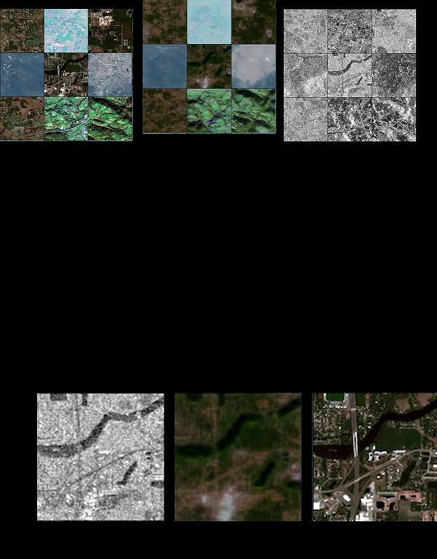
Figure 5 is another example of the actual generation of optical images, but I could not convert the images perfectly because some of the contours and topography of the original SAR images were missing.
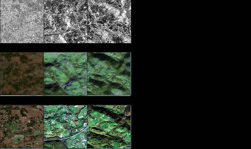
In some cases, as shown in the middle image, some of the information (the road in the lower left) could not be generated properly, or the colors of the field could not be extracted in detail. However, it was surprising that SAR images, which are completely different in appearance and nature from optical images, could be used to get a rough idea of the land situation and generate color images similar to RGB optical images.
(4) Conversion of optical image (grayscale) to optical image (RGB) using pix2pix
In this case, when converting from RGB to grayscale, it is necessary to load both of them simultaneously as a dataset. So you need to put the converted grayscale images together with the data loader and call it up at the time of training (the code is almost the same except for the following parts).
class ColorAndGray(object):
    def __call__(self, img):
        gray = img.convert('L')
        return img, gray

class MultiInputWrapper(object):
    def __init__(self, base_func):
        self.base_func = base_func

    def __call__(self, xs):
        if isinstance(self.base_func, list):
            return [f(x) for f,x in zip(self.base_func, xs)]
        else:
            return [self.base_func(x) for x in xs]

def load_datasets():
    transform  = transforms.Compose([
    ColorAndGray(),
    MultiInputWrapper(transforms.ToTensor()),
    MultiInputWrapper([
      transforms.Normalize(mean=(0.5,0.5,0.5,), std=(0.5,0.5,0.5,)),
      transforms.Normalize(mean=(0.5,), std=(0.5,))
    ])
  ])
    trainsets = datasets.ImageFolder(root = './GAN_datasets2',transform=transform)
    train_loader = torch.utils.data.DataLoader(trainsets, batch_size=128, num_workers=4, pin_memory=True)
    return train_loader
Training results
The following training results show the generator model at the 20 epochs when it was able to generate images most successfully (Figure 6) and the generator model at the 100 epochs (Figure 7). If you look closely at the result, you can see that although the RGB images converted by the generator at the 20 epochs have some tinting issues, they are generally colored as expected and reflect the forests, lakes, and roads in the actual optical image.
However, in Figure 7, in spite of much more training performed than Figure 6, spots and sheen appeared on parts of the lakes and roads that were not there, and the images could not be colored well.
To explore the cause of this, Figure 8 plots the loss of generators and discriminators for each epoch.
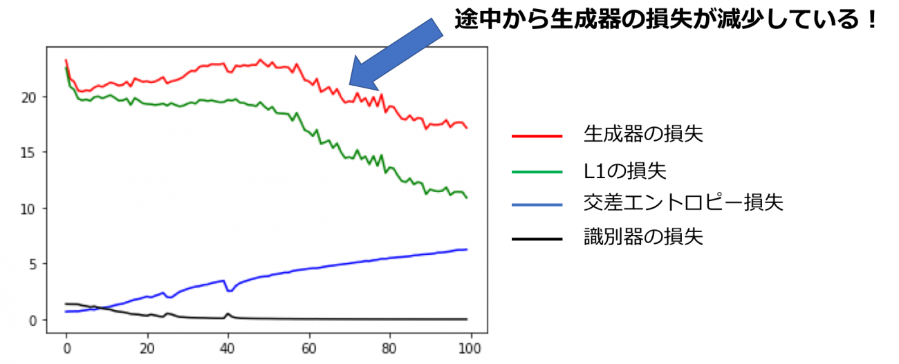
Ideally, during GAN training, the discriminator loss should decrease at each epoch, and the generator loss should increase with a small variance, but the above figure shows that the generator loss decreases after about 40 epochs. In short, this could be interpreted as “it may produce meaningless images after 40 epochs,” and the coloring results actually reflect this. Nevertheless, coloration was stable and fairly accurate while the losses of the generator were gradually increasing.
(5) Verification of PALSAR2 SAR images using the trained generator
Now that the generator for converting SAR image (grayscale) into optical image (RGB) and generator for converting optical image (grayscale) into optical image (RGB) have been built, I’d like to convert the grayscale image of PALSAR 2 available on Tellus to an RGB image.
The images used were L2.1 images of PALSAR 2 and extracted from the Lake Suwa area. Please refer to the following to find out how to extract the L2.1 products from PALSAR 2.
Tellus Takes on the Challenge of Calculating Land Coverage Using L2.1 Processing Data from PALSAR-2
The D. in Figure 9 is the actual input image to the generator. Compared to the original images like C., it is compressed into a 256×256 size image so that it can be passed through the generator. This is why some buildings, roads, and other detailed information are missing. As such, I examine how the generator behaves on SAR images with some missing information.
Generation results
Figure 10 shows the result when the HH polarized image of D. in Figure 9 was put into the generator.
Neither of them were able to make clear RGB images. Although the image produced with the generator for optical image (grayscale) to optical image (RGB) is slightly clearer in appearance, the image produced with the generator for SAR image to optical image seems to have a clearer distinction between Lake Suwa and the city area.
Although I was not able to convert SAR images to fine RGB optical images as I had originally hoped, I will continue to try further.
Next, I generate RGB images for both HH and HV polarized SAR images using two generators, and verify what results I get when combining them to create a pseudo-color image. The steps are as follows.
- Using the two generators built earlier, apply the RGB conversion process to the HH and HV polarized SAR images of 256×256.
2. Combine the generated images into a pseudo-color image (Red: HH polarisation, Green: HV polarisation, Blue: difference between HH and HV polarisation).
3. Compare the pseudo-color image created in step 2 with the original pseudo-color image made by combining the HH and HV polarized images before size reduction.
This allows us to compare the robustness to noise of the two generators built earlier and the properties of images stored.
Demonstration results
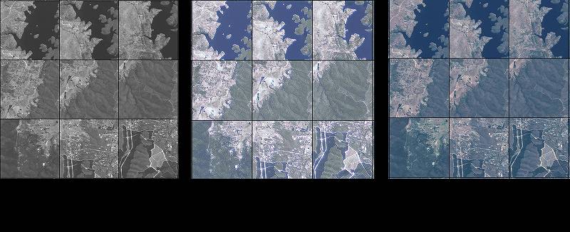
The results of the analysis performed according to the previous procedure are shown in Figure 11.
In terms of results, obviously the pseudo-color image before compressing the SAR image is the most beautiful. As for the SAR image that was compressed to fit into the pix2pix generator, the original information of the SAR image was retained in the generator for SAR image to optical image, while the generator for optical image (grayscale) to optical image (RGB) could not retain much information specific to SAR, resulting in a blurred image with noise.
From the above, it was found that the generator for SAR image to optical image was better able to generate images while preserving SAR-specific information than the generator for optical image (grayscale) to optical image (RGB).
(6) Future challenges
In this challenge, I trained the generators for SAR image (grayscale) to optical image (RGB) and for optical image (grayscale) to optical image (RGB) using pix2pix, a type of conditional GANs with conditions. I have also generated images from PALSAR 2, which is available on Tellus, in both generators and compared the specific differences between the two generators, and the following issues were identified.
– As the dataset used for the training included about 4,000 pairs of images only, further training with a larger number of images is necessary to make a full-scale demonstration.
– (Due to the dataset used,) while the images used in the training were of VV polarisation only, the actual test images were of HH and HV polarisation from PALSAR 2, which means that the types of polarisation images do not match.Therefore, verification should be conducted as soon as the VV polarized intensity images are available on Tellus.
– The images used in the training were SAR images taken from Sentinel-1, meaning that they were taken in the C-band. By contrast, PALSAR2 uses the L-band to capture images. Therefore, it is highly likely that the image information that takes into account differences in frequency bands has not been learned. In addition, since there is a difference in image resolution between PALSAR 2 and Sentinel-1, it is necessary to create a large number of PALSAR 2 image datasets for full-scale verification.
(7) Summary
It was not possible to convert SAR images to RGB optical images due to the differences in frequency bands and polarisation types of the SAR satellites.
However, it was confirmed that the generator trained to convert SAR images to optical images was less affected by noise in SAR images and tended to preserve more information about urban areas, etc. when the images generated from each type of polarisation were made into pseudo-color images.
With the development of these technologies, it may one day be possible to create RGB images from old SAR images or convert optical images into SAR images by creating and analyzing datasets that take into account the differences and characteristics of the satellite.