No Image Pair required! Converting To and From Optical and SAR Images With Unsupervised Learning
In this article we use a yet-to-be released data set to convert SAR images into optical images, and vise-versa by using unsupervised learning that doesn't require image pairs.
1. How to get started
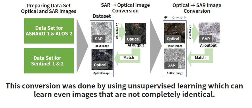
In this article we will convert SAR images into optical images, and vise-versa by using unsupervised learning that doesn’t require image pairs, as follows.
SAR allows us to take pictures of the earth without having to worry about the weather, and it is seeing increasingly more demand. However, since SAR is a special kind of sensor that is only used by satellites and airplanes, there is still only a limited amount of data available, making it very expensive to use. SAR is also different from your ordinary optical camera in that it uses electromagnetic waves to observe the earth’s surface, which makes it unsuitable for machine learning which requires a lot of data samples to run simulations.
In order to circumvent this, there are a lot of data scientists who convert optical images into SAR images, and vice-versa, by using supervised data. But still, there is a challenge even for these scientists. The main challenge is that it is very difficult to prepare image pairs that perfectly correspond with each other between optical and SAR images. To perfectly correspond means that the two pictures were taken under the same conditions, of the same location, and of the same thing. In order to get the ideal pair of two high quality images, the satellite would need to be equipped with both SAR and optical sensors, both with similar resolutions, both be taking pictures at the same time, and that data would need to be public. That isn’t something we can do just yet. Even if we had access to SAR and optical images that met these requirements, it would be really difficult to calibrate (match their positions ever so slightly to make sure they match up perfectly) them.
On the other hand, we have access to SAR and optical images that were taken with different resolutions and off-nadir angles of similar spots, which can be used for when they don’t have to match up perfectly. A pair of images taken by the ASNARO-1 (an optical satellite) and ALOS-2 (an SAR satellite) are an example of this. The only problem is that for these two satellites, the images specifications are so different that it couldn’t be considered a high-quality pair, making them difficult to conduct supervised learning on.
When that is the case, we can use unsupervised learning to try and convert between optical and SAR images, without using high-quality image pairs.
We will be attempting the following in this article.
– Collect a rough batch of ASNARO-1 (an optical satellite) and ALOS-2 (an SAR satellite) data, and convert between optical↔SAR images.
– Use a somewhat high-quality optical/SAR image pair (Sentinel-1, 2) to convert between optical↔SAR images.
– Compare the difference between supervised (Pix2Pix) and unsupervised (CycleGAN) learning to convert between optical↔SAR images.
2. Introduction of the Conversion Algorithm Technique
We will be using the Pix2Pix algorithm for supervised learning and the CycleGan algorithm for unsupervised learning. These two different techniques are primarily used to convert textures (not surface textures of patterns and colors) and are used together with another technology called GAN (Generative Adversarial Networks).
We talk about Pix2Pix in an article titled “Analyzing SAR Images Created With a Generator and Converting SAR Images Into Optical Images With Pix2Pix “, so we will only talk about CycleGAN in this article.
What makes CycleGAN (https://arxiv.org/abs/1703.10593) so great is that it makes texture conversion between two images possible without supervised learning. This is called domain conversion.
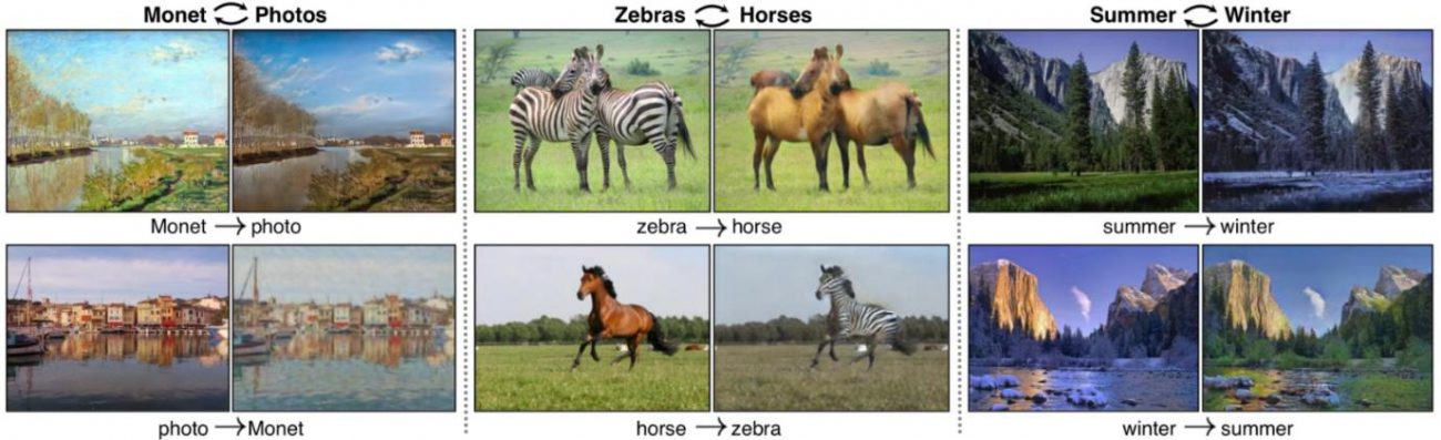
The most famous CycleGAN image is shown here, taken from an essay in which they discuss converting between a zebra and a horse. The only difference is that it changed the texture to make the horse into a zebra. This can also be applied to converting optical images into SAR images, where the only thing you have to change is the texture of what is being shown, without changing its contents.
This diagram, taken from the essay, explains the mechanism in more detail.
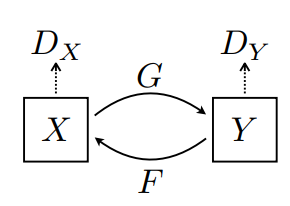
X is the zebra’s data set. Think of this as the zebra domain. Then we have Y, which is the horse’s data set. Think of this as the horse domain. For G, think of it as the device that converts the zebra into a horse. F is the opposite, it is the device that changes horses into zebras. GAN is Dx and Dy, or what’s called a discriminator, and is the machine that determines where other not the results of the conversion are accurate.
The optimized version of this is considered to be G(F(Y))=Y. This means that when you convert a horse into a zebra, and then back into a horse, you get the same horse that you started with, meaning that the input and output become a cycle. This is where the name “CycleGAN” comes from. In other words, when you have zebra=F(horse), horse=G(zebra), you get G(F(horse))=horse, and it cycles through the same input and output to become exactly alike.
If you can make two machines that cancel out the difference between the two domains (distributions), it would also be possible to do this for converting between optical and SAR images. To learn this unsupervised, we have to combine various loss functions, but we’ll cut out the in-depth explanation for this for now. For those of you who are interested, please read the original essay.
3. Preparing the Data Set
This time we will be using the following two data sets.
1) High-quality optical and SAR image pairs (Sentinel-1, 2)
2) ASNARO-1 (optical image) and ALOS-2 (SAR image) data
3.1. High quality optical and SAR image pairs (Sentinel-1, 2)
The first one is a data set that has been geometrically matched, taken by the Sentinel-1(SAR) and Sentinel-2 (optical) satellites. You can download it below.
https://mediatum.ub.tum.de/1436631
The entire file is very large (45GB), so you only need to download the folder titled “ROIs1970_fall” for this article.
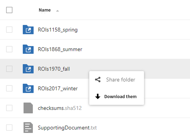
When the download is complete on the development environment, run the following to unzip the data.
$ unzip ROIs1970_fall
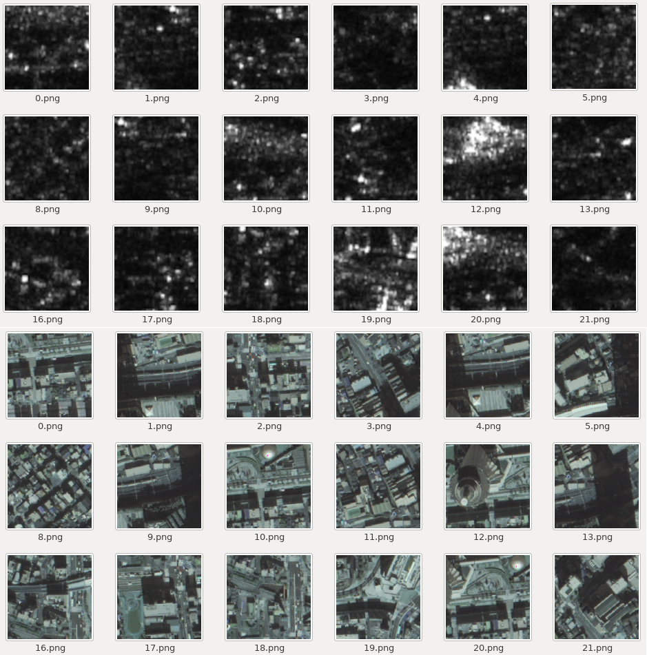
Unzipping the folder will give you a series of folders titled: s1_1, s1_2, s1_3…, s2_1, s2_2, s2_3…, etc. Folders with s1 in their name are SAR images, and those with s2 in their name are the optical images. All of the images are 256px, and the SAR images are VV polarized.
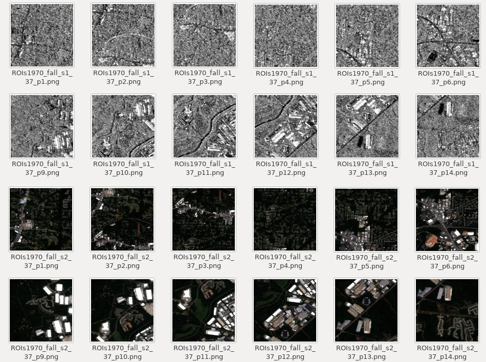
These pairs of SAR and optical images are of very high quality, so we should be able to convert between them.
They are already in a pair, so in order to use them for unsupervised learning, we will have to use them without pairing them.
3.2. ASNARO-1 (optical image) and ALOS-2 (SAR image) Data
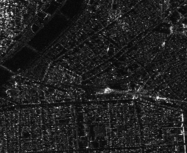
Next, we will build the second set of data ourselves on the Tellus environment. First, we will acquire SAR L2.1 images from ALOS-2 of Tokyo Skytree tower.
import os, requests
import geocoder # ! pip install geocoder

# Fields
BASE_API_URL = "https://file.tellusxdp.com/api/v1/origin/search/" # https://www.tellusxdp.com/docs/api-reference/palsar2-files-v1.html#/
ACCESS_TOKEN = "ご自身のトークンを貼り付けてください"
HEADERS = {"Authorization": "Bearer " + ACCESS_TOKEN}
TARGET_PLACE = "Skytree, Tokyo"
SAVE_DIRECTORY="./data/"

# Functions
def rect_vs_point(ax, ay, aw, ah, bx, by):
    return 1 if bx > ax and bx  ay and by < ah else 0

def get_scene_list(_get_params={}):
    query = "palsar2-l21"
    r = requests.get(BASE_API_URL + query, _get_params, headers=HEADERS)
    if not r.status_code == requests.codes.ok:
        r.raise_for_status()
    return r.json()

def get_scenes(_target_json, _get_params={}):
    # get file list
    r = requests.get(_target_json["publish_link"], _get_params, headers=HEADERS)
    if not r.status_code == requests.codes.ok:
        r.raise_for_status()
    file_list = r.json()['files']
    dataset_id = _target_json['dataset_id'] # folder name
    # make dir
    if os.path.exists(SAVE_DIRECTORY + dataset_id) == False:
        os.makedirs(SAVE_DIRECTORY + dataset_id)
    # downloading
    print("[Start downloading]", dataset_id)
    for _tmp in file_list:
        r = requests.get(_tmp['url'], headers=HEADERS, stream=True)
        if not r.status_code == requests.codes.ok:
            r.raise_for_status()
        with open(os.path.join(SAVE_DIRECTORY, dataset_id, _tmp['file_name']), "wb") as f:
            f.write(r.content)
        print("  - [Done]", _tmp['file_name'])
    print("finished")
    return

# Entry point
def main():
    # extract slc list around the address
    gc = geocoder.osm(TARGET_PLACE, timeout=5.0) # get latlon
    #print(gc.latlng)
    scene_list_json = get_scene_list({"page_size":"1000", "mode":"SM1", "left_bottom_lat":  gc.latlng[0], "left_bottom_lon":  gc.latlng[1], "right_top_lat":  gc.latlng[0], "right_top_lon":  gc.latlng[1]})
    #print(scene_list_json["count"])
    target_places_json = [_ for _ in scene_list_json['items'] if rect_vs_point(_['bbox'][1], _['bbox'][0], _['bbox'][3], _['bbox'][2], gc.latlng[0], gc.latlng[1])] # lot_min, lat_min, lot_max...
    #print(target_places_json)
    target_ids = [_['dataset_id'] for _ in target_places_json]
    print("[Matched SLCs]", target_ids)
    # download
    for target_id in target_ids:
        target_json = [_ for _ in scene_list_json['items'] if _['dataset_id'] == target_id][0]
        # download the target file
        get_scenes(target_json)

if __name__=="__main__":
       main()
When you run it, the following 2 images will be applicable and will be saved in the data folder.
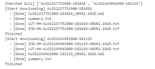
Now we will explain the important parts of the code.
scene_list_json = get_scene_list({"page_size":"1000", "mode":"SM1", "left_bottom_lat": gc.latlng[0], "left_bottom_lon": gc.latlng[1], "right_top_lat": gc.latlng[0], "right_top_lon": gc.latlng[1]})Here we can use the Tellus API to check if there is a SAR image that matches our conditions. Our conditions are that the image contains Skytree, and that it is set to SM1. SM1 is a SAR observational mode called Stripmap1, with a resolution of 3m. The SAR images that you download have latitude and longitude information in addition to the “GeoTiff” pixel value.
Next, we will extract a portion of the SAR image that we want to use. In order to do this, we trim the image using longitude and latitude, and if we look up the GeoTiff we downloaded as a $gdalinfo file, it should be ESPG:9001 as follows.
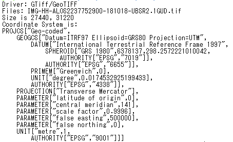
Using a software that specializes in processing Geotiff and other files called GDAL, it is hard to trim the image at EPSG:9001, so use the program below to change the projection system to ESPG:4326 before you trim the image.
import os, requests, subprocess
from osgeo import gdal
from osgeo import gdal_array

# Entry point
def main():
    cmd = "find ./data/ALOS* | grep tif"
    process = (subprocess.Popen(cmd, stdout=subprocess.PIPE,shell=True).communicate()[0]).decode('utf-8')
    file_name_list = process.rsplit()
    for _file_name in file_name_list:
        convert_file_name =   _file_name + "_converted.tif"
        crop_file_name =   _file_name + "_cropped.tif"
        x1 = 139.807069
        y1 = 35.707233
        x2 = 139.814111
        y2 = 35.714069
        cmd = 'gdalwarp -t_srs EPSG:4326 ' +_file_name + ' ' + convert_file_name
        process = (subprocess.Popen(cmd, stdout=subprocess.PIPE,shell=True).communicate()[0]).decode('utf-8')
        print("[Done] ", convert_file_name)
        cmd = 'gdal_translate -projwin ' + str(x1) + ' ' + str(y1) + ' ' +  str(x2) + ' ' + str(y2) + ' ' + convert_file_name + " " + crop_file_name
        print(cmd)
        process = (subprocess.Popen(cmd, stdout=subprocess.PIPE,shell=True).communicate()[0]).decode('utf-8')
        print("[Done] ", crop_file_name)

if __name__=="__main__":
       main()
When you have finished this step, you should have the following files.

The data we will be using today ends with “cropped.tif”.
Now that you have a SAR image of the area around Tokyo Skytree, let’s dig into the important parts of the code we will be using.
Below, we are converting the coordinate system using a software called GDAL.
cmd = 'gdalwarp -t_srs EPSG:4326 ' +_file_name + ' ' + convert_file_nameNext, we crop the image around Tokyo Skytree using the GDAL software.
cmd = 'gdal_translate -projwin ' + str(x1) + ' ' + str(y1) + ' ' + str(x2) + ' ' + str(y2) + ' ' + convert_file_name + " " + crop_file_nameAnd now your SAR image is ready. Next, we need to find an optical image taken by ASNARO-1 that matches our cropped Skytree image. Let’s try running the following code.
import os, requests
import geocoder # ! pip install geocoder
import math
from skimage import io
from io import BytesIO
import numpy as np
import cv2

# Fields
BASE_API_URL = "https://gisapi.tellusxdp.com"
ASNARO1_SCENE = "/api/v1/asnaro1/scene"
ACCESS_TOKEN = "ご自身のトークンを貼り付けてください"
HEADERS = {"Authorization": "Bearer " + ACCESS_TOKEN}
TARGET_PLACE = "skytree, Tokyo"
SAVE_DIRECTORY="./data/asnaro/"
ZOOM_LEVEL=18
IMG_SYNTH_NUM=6
IMG_BASE_SIZE=256

# Functions
def get_tile_num(lat_deg, lon_deg, zoom):
    lat_rad = math.radians(lat_deg)
    n = 2.0 ** zoom
    xtile = int((lon_deg + 180.0) / 360.0 * n)
    ytile = int((1.0 - math.log(math.tan(lat_rad) + (1 / math.cos(lat_rad))) / math.pi) / 2.0 * n)
    return (xtile, ytile)

def get_scene_list(_get_params={}):
    query = BASE_API_URL + ASNARO1_SCENE
    r = requests.get(query, _get_params, headers=HEADERS)
    if not r.status_code == requests.codes.ok:
        r.raise_for_status()
    return r.json()

def get_scene(_id, _xc, _yc):
    # mkdir
    save_file_name = SAVE_DIRECTORY + _id + ".png"
    if os.path.exists(SAVE_DIRECTORY) == False:
        os.makedirs(SAVE_DIRECTORY)

    # download
    save_image = np.zeros((IMG_SYNTH_NUM * IMG_BASE_SIZE, IMG_SYNTH_NUM * IMG_BASE_SIZE, 3))
    for i in range(IMG_SYNTH_NUM):
        for j in range(IMG_SYNTH_NUM):
            query = "/ASNARO-1/" + _id + "/" + str(ZOOM_LEVEL) + "/" + str(_xc-int(IMG_SYNTH_NUM*0.5)+i) + "/" + str(_yc-int(IMG_SYNTH_NUM*0.5)+j) + ".png"
            r = requests.get(BASE_API_URL + query, headers=HEADERS)
            if not r.status_code == requests.codes.ok:
                r.raise_for_status()
            img = io.imread(BytesIO(r.content))
            save_image[i*IMG_BASE_SIZE:(i+1)*IMG_BASE_SIZE, j*IMG_BASE_SIZE:(j+1)*IMG_BASE_SIZE, :] = img[:, :, 0:3].transpose(1, 0, 2) # [x, y, c] -> [y, x, c]
    save_image = cv2.flip(save_image, 1)
    save_image = cv2.rotate(save_image, cv2.ROTATE_90_COUNTERCLOCKWISE)
    cv2.imwrite(save_file_name, save_image)
    print("[DONE]" + save_file_name)
    return


# Entry point
def main():
    # extract slc list around the address
    gc = geocoder.osm(TARGET_PLACE, timeout=5.0) # get latlon
    scene_list = get_scene_list({"min_lat":  gc.latlng[0], "min_lon":  gc.latlng[1], "max_lat":  gc.latlng[0], "max_lon":  gc.latlng[1]})
    for _scene in scene_list:
        #_xc, _yc = get_tile_num(_scene['clat'], _scene['clon'], ZOOM_LEVEL) # center
        _xc, _yc = get_tile_num(gc.latlng[0], gc.latlng[1], ZOOM_LEVEL)
        get_scene(_scene['entityId'], _xc, _yc)

if __name__=="__main__":
       main()
Performing this code gives you the following.
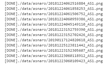
This should give you data for the area around Skytree taken by ASNARO-1. ASNARO-1’s API is limited to images uploaded via patches on Tellus, so once you have found data that contains Tokyo Skytree, you’ll have to collect the patches around it to make the image you need. Therefore, it is possible to obtain the following – a single image of a wide area in high resolution.
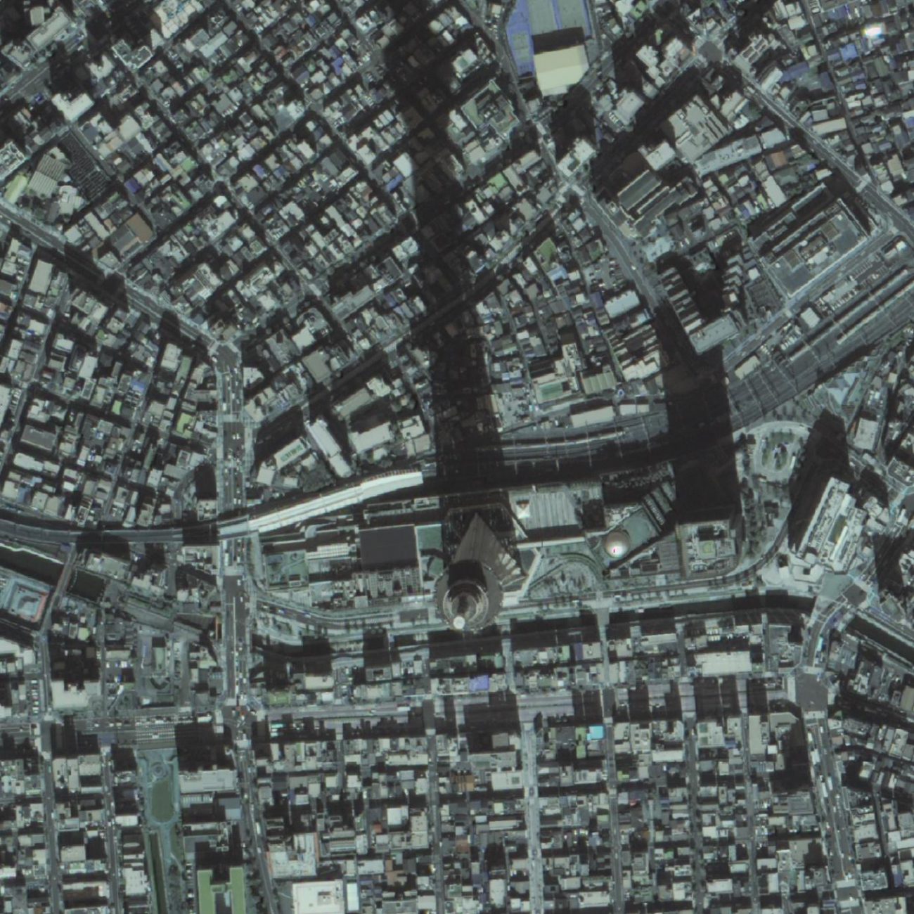
Depending on the angle, it may look like the Skytree has fallen over, so try to avoid images where it doesn’t look like this, as well as images that don’t contain blur or noise.
Okay, let’s dig into the important parts of the code we will be using for this part.
Below is a list of observational data taken by ASNARO-1 where the Skytree has been captured.
scene_list = get_scene_list({"min_lat": gc.latlng[0], "min_lon": gc.latlng[1], "max_lat": gc.latlng[0], "max_lon": gc.latlng[1]})We have gathered patch images of Skytree below.
        _xc, _yc = get_tile_num(gc.latlng[0], gc.latlng[1], ZOOM_LEVEL)
        get_scene(_scene['entityId'], _xc, _yc)
Of all of the get_scene functions, you may find the following process a little strange.
            save_image[i*IMG_BASE_SIZE:(i+1)*IMG_BASE_SIZE, j*IMG_BASE_SIZE:(j+1)*IMG_BASE_SIZE, :] = img[:, :, 0:3].transpose(1, 0, 2) # [x, y, c] -> [y, x, c]
    save_image = cv2.flip(save_image, 1)
    save_image = cv2.rotate(save_image, cv2.ROTATE_90_COUNTERCLOCKWISE)
This is because the resulting patch images are x, y, c, but if you export in OpenCV, they will be converted to something you must treat as y, x, c, so we have the conversion process written in there as well. They have also been rotated so they are zoomed in to the north as the SAR images.
With this, you have the same optical images as you do SAR images. You could perform machine learning with what you have now, but you wouldn’t get results that you would be able to confirm with your own eyes, so we will do a quick matching process to help with that.
The resolution of the SAR images taken by ALOS-2 is 3m, and the resolution of the multi-images taken by ASNARO-1 is 2m, and both have been taken under different conditions, with different off-nadir angles. This makes it impossible for them to match up perfectly, so we will do an easy process to make them roughly line up.
The matching process uses the following code. (source: https://qiita.com/suuungwoo/items/9598cbac5adf5d5f858e) This time we will be using a method called “AKAZE” to scale, shift, and rotate the images, which is a really good matching process algorithm.
import cv2

float_img = cv2.imread('data/ALOS2237752900-181018/IMG-HH-ALOS2237752900-181018-UBSR2.1GUD.tif_cropped.tif', cv2.IMREAD_GRAYSCALE)
ref_img = cv2.imread('data/asnaro/20181224060959386_AS1.png', cv2.IMREAD_GRAYSCALE)

akaze = cv2.AKAZE_create()
float_kp, float_des = akaze.detectAndCompute(float_img, None)
ref_kp, ref_des = akaze.detectAndCompute(ref_img, None)
bf = cv2.BFMatcher()
matches = bf.knnMatch(float_des, ref_des, k=2)
good_matches = []
for m, n in matches:
    if m.distance < 0.95 * n.distance:
        good_matches.append([m])

matches_img = cv2.drawMatchesKnn(
    float_img,
    float_kp,
    ref_img,
    ref_kp,
    good_matches,
    None,
    flags=cv2.DrawMatchesFlags_NOT_DRAW_SINGLE_POINTS)
cv2.imwrite('matches.png', matches_img)
When you run it, you should get the following.
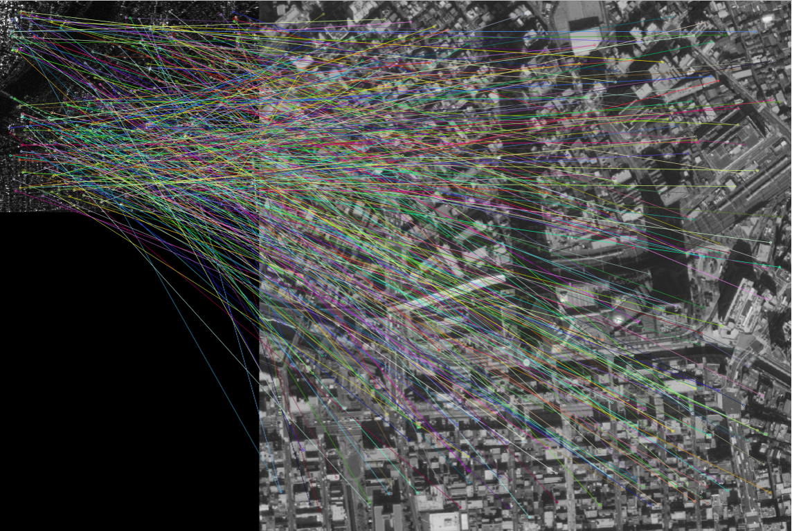
This matching data will work as a rough match that you can fine-tune manually. As a result you should get the following two image pairs.
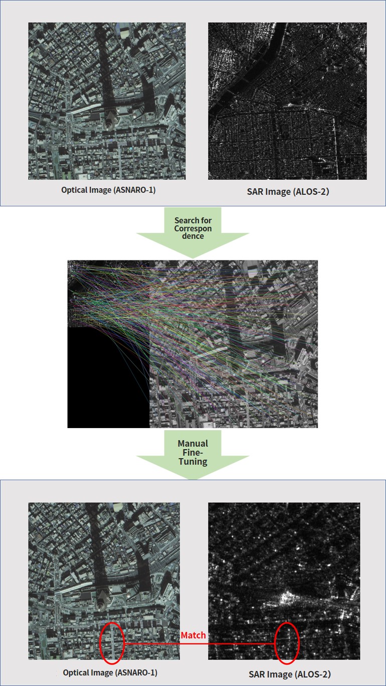
Looking at the two images, you may feel like they have both changed completely, but the position of the roads, how big they are, and such, should match up. There is still a big difference in their resolutions though, and it is harder to make out the buildings in the SAR image.
To fix this we have prepared the following two sets of data.
1.High-Quality Optical and SAR Image Pairs (Sentinel-1, 2)
2.ASNARO-1 (optical image) and ALOS-2 (SAR image) Data
Now we are ready to finally start the machine learning.
4. Converting Between Optical↔SAR Images With Unsupervised Learning (CycleGen)
You can get what you need for CycleGAN from this link: https://github.com/eriklindernoren/Keras-GAN/tree/master/cyclegan
*Please be sure to read everything because there are programs used to read the data that can be used for both conversions.
4.1. High-Quality Optical and SAR Image Pairs (Sentinel-1, 2)
We will start by testing out the above mentioned data set.
First, create a folder titled “$mkdir your_workfolder” that you will use to run the program, and use it as a route directory and do all of your work in this folder. It should look like the following if you follow the process and run the program correctly. If there is something different you may have to go back and check if there is something wrong.
root
|- cyclegan.py
|- data_loader_py
|- datasets
| |- sat
| |-testA
| | |- file...
| |-testB
| | |- file...
| |-trainA
| | |- file...
| |-trainB
| |- file...
|- data_split.py
|- images
| |- sar
| |- file…
|- ROIs1970_fall (どこに設置しても良い)
In order to split the ROIs1970_fal data into two domains (optical and SAR), you’ll run the following code. Save it as data_split.py.
import os, requests, subprocess
import math
import numpy as np
import cv2
import random

# read dataset
file_path = "./ROIs1970_fall/"
cmd = "find " + file_path + "s1* | grep png"
process = (subprocess.Popen(cmd, stdout=subprocess.PIPE,shell=True).communicate()[0]).decode('utf-8')
file_name_list = process.rsplit()
data_x = []
data_y = []
for _file_name in file_name_list:
  data_x.append(_file_name)
  data_y.append(_file_name.replace('s1_','s2_'))
data_x = np.asarray(data_x)
data_y = np.asarray(data_y)

# extract data
part_data_ratio = 0.1 # extract data depending on the ratio from all data
test_data_ratio = 0.1
all_data_size = len(data_x)
idxs = range(all_data_size) # all data
part_idxs = random.sample(idxs, int(all_data_size * part_data_ratio)) # part data
part_data_size = len(part_idxs)
test_data_idxs = random.sample(part_idxs, int(part_data_size * test_data_ratio)) # test data from part data
train_data_idxs = list(set(part_idxs) - set(test_data_idxs)) # train data = all data - test data
test_x = data_x[test_data_idxs]
test_y = data_y[test_data_idxs]
train_x = data_x[train_data_idxs]
train_y = data_y[train_data_idxs]

# data copy
os.makedirs('datasets/sar/trainA', exist_ok=True)
os.makedirs('datasets/sar/trainB', exist_ok=True)
os.makedirs('datasets/sar/testA', exist_ok=True)
os.makedirs('datasets/sar/testB', exist_ok=True)
cmd = 'find ./datasets/sar/* -type l -exec unlink {} ;'
process = (subprocess.Popen(cmd, stdout=subprocess.PIPE,shell=True).communicate()[0]).decode('utf-8')
print("[Start] extract test dataset")
for i in range(len(test_x)):
  cmd = "ln -s " + test_x[i] + " datasets/sar/testA/"
  process = (subprocess.Popen(cmd, stdout=subprocess.PIPE,shell=True).communicate()[0]).decode('utf-8')
  cmd = "ln -s " + test_y[i] + " datasets/sar/testB/"
  process = (subprocess.Popen(cmd, stdout=subprocess.PIPE,shell=True).communicate()[0]).decode('utf-8')
  if i % 500 == 0:
    print("[Done] ", i, "/", len(test_x))
print("Finished")

print("[Start] extract train dataset")
for i in range(len(train_x)):
  cmd = "ln -s " + train_x[i] + " datasets/sar/trainA/"
  process = (subprocess.Popen(cmd, stdout=subprocess.PIPE,shell=True).communicate()[0]).decode('utf-8')
  cmd = "ln -s " + train_y[i] + " datasets/sar/trainB/"
  process = (subprocess.Popen(cmd, stdout=subprocess.PIPE,shell=True).communicate()[0]).decode('utf-8')
  if i % 500 == 0:
    print("[Done] ", i, "/", len(train_x))
print("Finished")
If you run this, the ./datasets/sar/ array will create the folders “trainA, trainB, testA, testB”, splitting up the domain images for you. A is the SAR domain, and B is the optical domain.
The data loader program for loading the created image can be found below. Break them down into levels by saving them with the name to “data_loader.py”. They will be used for a different program we will get into later, so make sure to correctly set up their levels.
import scipy
from glob import glob
import numpy as np

class DataLoader():
    def __init__(self, dataset_name, img_res=(256, 256)):
        self.dataset_name = dataset_name
        self.img_res = img_res

    def load_data(self, domain, batch_size=1, is_testing=False):
        data_type = "train%s" % domain if not is_testing else "test%s" % domain
        path = glob('./datasets/%s/%s/*' % (self.dataset_name, data_type))

        batch_images = np.random.choice(path, size=batch_size)

        imgs = []
        for img_path in batch_images:
            img = self.imread(img_path)
            if not is_testing:
                img = scipy.misc.imresize(img, self.img_res)

                if np.random.random() > 0.5:
                    img = np.fliplr(img)
            else:
                img = scipy.misc.imresize(img, self.img_res)
            imgs.append(img)

        imgs = np.array(imgs)/127.5 - 1.
        return imgs

    def load_data_with_label(self, domain, batch_size=1, is_testing=False):
        data_type = "train%s" % domain if not is_testing else "test%s" % domain
        path = glob('./datasets/%s/%s/*' % (self.dataset_name, data_type))

        batch_images = np.random.choice(path, size=batch_size)

        imgs = []
        lbls = []
        for img_path in batch_images:
            img = self.imread(img_path)
            # lbl path
            if "A/" in img_path:
              lbl_path = img_path.replace('s1_', 's2_')
              lbl_path = lbl_path.replace('A/', 'B/')
            else:
              lbl_path = img_path.replace('s2_', 's1_')
              lbl_path = lbl_path.replace('B/', 'A/')
            lbl = self.imread(lbl_path)

            if not is_testing:
                img = scipy.misc.imresize(img, self.img_res)
                lbl = scipy.misc.imresize(lbl, self.img_res)

                if np.random.random() > 0.5:
                    img = np.fliplr(img)
                    lbl = np.fliplr(lbl)
            else:
                img = scipy.misc.imresize(img, self.img_res)
                lbl = scipy.misc.imresize(lbl, self.img_res)
            imgs.append(img)
            lbls.append(lbl)
        imgs = np.array(imgs)/127.5 - 1.
        lbls = np.array(lbls)/127.5 - 1.
        return imgs, lbls


    def load_batch(self, batch_size=1, is_testing=False):
        data_type = "train" if not is_testing else "val"
        path_A = glob('./datasets/%s/%sA/*' % (self.dataset_name, data_type))
        path_B = glob('./datasets/%s/%sB/*' % (self.dataset_name, data_type))

        self.n_batches = int(min(len(path_A), len(path_B)) / batch_size)
        total_samples = self.n_batches * batch_size

        # Sample n_batches * batch_size from each path list so that model sees all
        # samples from both domains
        path_A = np.random.choice(path_A, total_samples, replace=False)
        path_B = np.random.choice(path_B, total_samples, replace=False)

        for i in range(self.n_batches-1):
            batch_A = path_A[i*batch_size:(i+1)*batch_size]
            batch_B = path_B[i*batch_size:(i+1)*batch_size]
            imgs_A, imgs_B = [], []
            for img_A, img_B in zip(batch_A, batch_B):
                img_A = self.imread(img_A)
                img_B = self.imread(img_B)

                img_A = scipy.misc.imresize(img_A, self.img_res)
                img_B = scipy.misc.imresize(img_B, self.img_res)

                if not is_testing and np.random.random() > 0.5:
                        img_A = np.fliplr(img_A)
                        img_B = np.fliplr(img_B)

                imgs_A.append(img_A)
                imgs_B.append(img_B)

            imgs_A = np.array(imgs_A)/127.5 - 1.
            imgs_B = np.array(imgs_B)/127.5 - 1.

            yield imgs_A, imgs_B

    def load_img(self, path):
        img = self.imread(path)
        img = scipy.misc.imresize(img, self.img_res)
        img = img/127.5 - 1.
        return img[np.newaxis, :, :, :]

    def imread(self, path):
        return scipy.misc.imread(path, mode='RGB').astype(np.float)
This program will be used every time you run learning with CycleGan. The SAR and optical image data is saved as imgs_A and imgs_B. Now we will get to the actual CycleGAN program. Save it as “cyclegan.py” in the first level.
from __future__ import print_function, division
import scipy

from keras.datasets import mnist
from keras_contrib.layers.normalization.instancenormalization import InstanceNormalization
from keras.layers import Input, Dense, Reshape, Flatten, Dropout, Concatenate
from keras.layers import BatchNormalization, Activation, ZeroPadding2D
from keras.layers.advanced_activations import LeakyReLU
from keras.layers.convolutional import UpSampling2D, Conv2D
from keras.models import Sequential, Model
from tensorflow.keras.optimizers import Adam
import datetime
import sys
from data_loader import DataLoader
import numpy as np
import os
import matplotlib as mpl
mpl.use('Agg')
import matplotlib.pyplot as plt

class CycleGAN():
    def __init__(self):
        # Input shape
        self.img_rows = 256
        self.img_cols = 256
        self.channels = 3
        self.img_shape = (self.img_rows, self.img_cols, self.channels)

        # Configure data loader
        self.dataset_name = 'sar'
        self.data_loader = DataLoader(dataset_name=self.dataset_name,
                                      img_res=(self.img_rows, self.img_cols))


        # Calculate output shape of D (PatchGAN)
        patch = int(self.img_rows / 2**4)
        self.disc_patch = (patch, patch, 1)

        # Number of filters in the first layer of G and D
        self.gf = 64
        self.df = 64

        # Loss weights
        self.lambda_cycle = 10.0                    # Cycle-consistency loss
        self.lambda_id = 0.1 * self.lambda_cycle    # Identity loss

        optimizer = Adam(0.0002, 0.5)

        # Build and compile the discriminators
        self.d_A = self.build_discriminator()
        self.d_B = self.build_discriminator()
        self.d_A.compile(loss='mse',
            optimizer=optimizer,
            metrics=['accuracy'])
        self.d_B.compile(loss='mse',
            optimizer=optimizer,
            metrics=['accuracy'])

        #-------------------------
        # Construct Computational
        #   Graph of Generators
        #-------------------------

        # Build the generators
        self.g_AB = self.build_generator()
        self.g_BA = self.build_generator()

        # Input images from both domains
        img_A = Input(shape=self.img_shape)
        img_B = Input(shape=self.img_shape)

        # Translate images to the other domain
        fake_B = self.g_AB(img_A)
        fake_A = self.g_BA(img_B)
        # Translate images back to original domain
        reconstr_A = self.g_BA(fake_B)
        reconstr_B = self.g_AB(fake_A)
        # Identity mapping of images
        img_A_id = self.g_BA(img_A)
        img_B_id = self.g_AB(img_B)

        # For the combined model we will only train the generators
        self.d_A.trainable = False
        self.d_B.trainable = False

        # Discriminators determines validity of translated images
        valid_A = self.d_A(fake_A)
        valid_B = self.d_B(fake_B)

        # Combined model trains generators to fool discriminators
        self.combined = Model(inputs=[img_A, img_B],
                              outputs=[ valid_A, valid_B,
                                        reconstr_A, reconstr_B,
                                        img_A_id, img_B_id ])
        self.combined.compile(loss=['mse', 'mse',
                                    'mae', 'mae',
                                    'mae', 'mae'],
                            loss_weights=[  1, 1,
                                            self.lambda_cycle, self.lambda_cycle,
                                            self.lambda_id, self.lambda_id ],
                            optimizer=optimizer)

    def build_generator(self):
        """U-Net Generator"""

        def conv2d(layer_input, filters, f_size=4):
            """Layers used during downsampling"""
            d = Conv2D(filters, kernel_size=f_size, strides=2, padding='same')(layer_input)
            d = LeakyReLU(alpha=0.2)(d)
            d = InstanceNormalization()(d)
            return d

        def deconv2d(layer_input, skip_input, filters, f_size=4, dropout_rate=0):
            """Layers used during upsampling"""
            u = UpSampling2D(size=2)(layer_input)
            u = Conv2D(filters, kernel_size=f_size, strides=1, padding='same', activation='relu')(u)
            if dropout_rate:
                u = Dropout(dropout_rate)(u)
            u = InstanceNormalization()(u)
            u = Concatenate()([u, skip_input])
            return u

        # Image input
        d0 = Input(shape=self.img_shape)

        # Downsampling
        d1 = conv2d(d0, self.gf)
        d2 = conv2d(d1, self.gf*2)
        d3 = conv2d(d2, self.gf*4)
        d4 = conv2d(d3, self.gf*8)

        # Upsampling
        u1 = deconv2d(d4, d3, self.gf*4)
        u2 = deconv2d(u1, d2, self.gf*2)
        u3 = deconv2d(u2, d1, self.gf)

        u4 = UpSampling2D(size=2)(u3)
        output_img = Conv2D(self.channels, kernel_size=4, strides=1, padding='same', activation='tanh')(u4)

        return Model(d0, output_img)

    def build_discriminator(self):

        def d_layer(layer_input, filters, f_size=4, normalization=True):
            """Discriminator layer"""
            d = Conv2D(filters, kernel_size=f_size, strides=2, padding='same')(layer_input)
            d = LeakyReLU(alpha=0.2)(d)
            if normalization:
                d = InstanceNormalization()(d)
            return d

        img = Input(shape=self.img_shape)

        d1 = d_layer(img, self.df, normalization=False)
        d2 = d_layer(d1, self.df*2)
        d3 = d_layer(d2, self.df*4)
        d4 = d_layer(d3, self.df*8)

        validity = Conv2D(1, kernel_size=4, strides=1, padding='same')(d4)

        return Model(img, validity)

    def train(self, epochs, batch_size=1, sample_interval=50):

        start_time = datetime.datetime.now()

        # Adversarial loss ground truths
        valid = np.ones((batch_size,) + self.disc_patch)
        fake = np.zeros((batch_size,) + self.disc_patch)

        for epoch in range(epochs):
            for batch_i, (imgs_A, imgs_B) in enumerate(self.data_loader.load_batch(batch_size)):

                # ----------------------
                #  Train Discriminators
                # ----------------------

                # Translate images to opposite domain
                fake_B = self.g_AB.predict(imgs_A)
                fake_A = self.g_BA.predict(imgs_B)

                # Train the discriminators (original images = real / translated = Fake)
                dA_loss_real = self.d_A.train_on_batch(imgs_A, valid)
                dA_loss_fake = self.d_A.train_on_batch(fake_A, fake)
                dA_loss = 0.5 * np.add(dA_loss_real, dA_loss_fake)

                dB_loss_real = self.d_B.train_on_batch(imgs_B, valid)
                dB_loss_fake = self.d_B.train_on_batch(fake_B, fake)
                dB_loss = 0.5 * np.add(dB_loss_real, dB_loss_fake)

                # Total disciminator loss
                d_loss = 0.5 * np.add(dA_loss, dB_loss)


                # ------------------
                #  Train Generators
                # ------------------

                # Train the generators
                g_loss = self.combined.train_on_batch([imgs_A, imgs_B],
                                                        [valid, valid,
                                                        imgs_A, imgs_B,
                                                        imgs_A, imgs_B])

                elapsed_time = datetime.datetime.now() - start_time

                # Plot the progress
                print ("[Epoch %d/%d] [Batch %d/%d] [D loss: %f, acc: %3d%%] [G loss: %05f, adv: %05f, recon: %05f, id: %05f] time: %s "
                                                                        % ( epoch, epochs,
                                                                            batch_i, self.data_loader.n_batches,
                                                                            d_loss[0], 100*d_loss[1],
                                                                            g_loss[0],
                                                                            np.mean(g_loss[1:3]),
                                                                            np.mean(g_loss[3:5]),
                                                                            np.mean(g_loss[5:6]),
                                                                            elapsed_time))

                # If at save interval => save generated image samples
                if batch_i % sample_interval == 0:
                    self.sample_images(epoch, batch_i)

    def sample_images(self, epoch, batch_i):
        os.makedirs('images/%s' % self.dataset_name, exist_ok=True)
        r, c = 2, 4

        imgs_A, lbls_A = self.data_loader.load_data_with_label(domain="A", batch_size=1, is_testing=True)
        imgs_B, lbls_B = self.data_loader.load_data_with_label(domain="B", batch_size=1, is_testing=True)

        # Translate images to the other domain
        fake_B = self.g_AB.predict(imgs_A)
        fake_A = self.g_BA.predict(imgs_B)
        # Translate back to original domain
        reconstr_A = self.g_BA.predict(fake_B)
        reconstr_B = self.g_AB.predict(fake_A)

        gen_imgs = np.concatenate([imgs_A, fake_B, reconstr_A, lbls_A, imgs_B, fake_A, reconstr_B, lbls_B])

        # Rescale images 0 - 1
        gen_imgs = 0.5 * gen_imgs + 0.5

        titles = ['Original', 'Translated', 'Reconstructed', 'Label']
        fig, axs = plt.subplots(r, c)
        cnt = 0
        for i in range(r):
            for j in range(c):
                axs[i,j].imshow(gen_imgs[cnt])
                axs[i, j].set_title(titles[j])
                axs[i,j].axis('off')
                cnt += 1

        fig.savefig("images/%s/%d_%d.png" % (self.dataset_name, epoch, batch_i))
        plt.close()


if __name__ == '__main__':
    gan = CycleGAN()
    gan.train(epochs=200, batch_size=1, sample_interval=200)
Performing this code gives you the following.
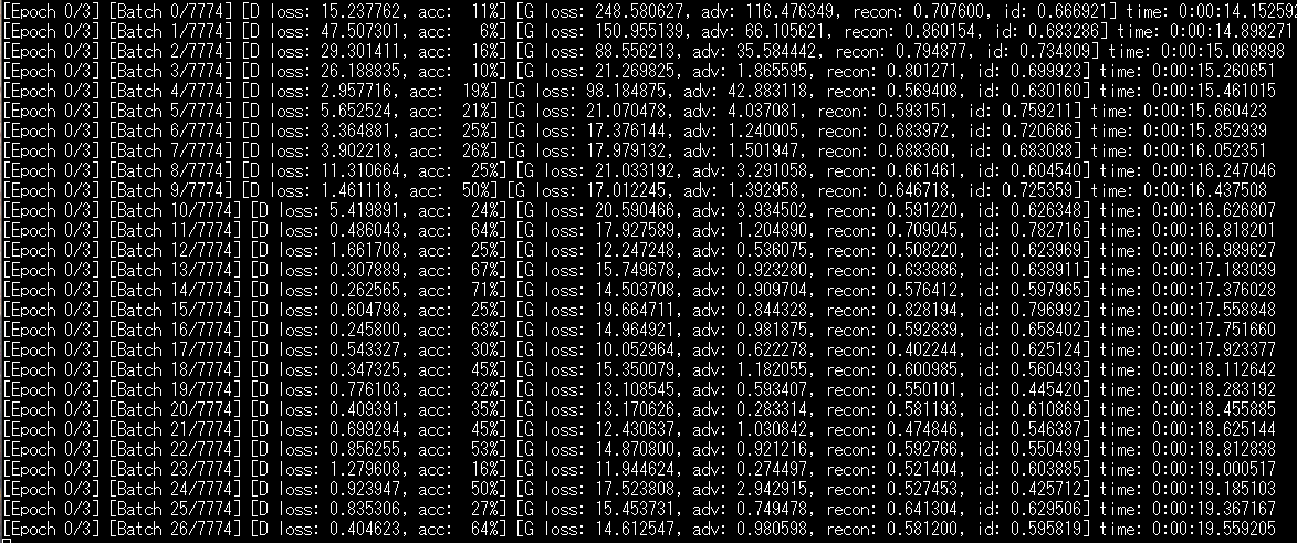
We will give a quick explanation of the code. We are conducting learning on the following parts. Every time it is opened, it takes data from the data loader.
g_loss = self.combined.train_on_batch([imgs_A, imgs_B],
                                                        [valid, valid,
                                                        imgs_A, imgs_B,
                                                        imgs_A, imgs_B])
                elapsed_time = datetime.datetime.now() - start_time))
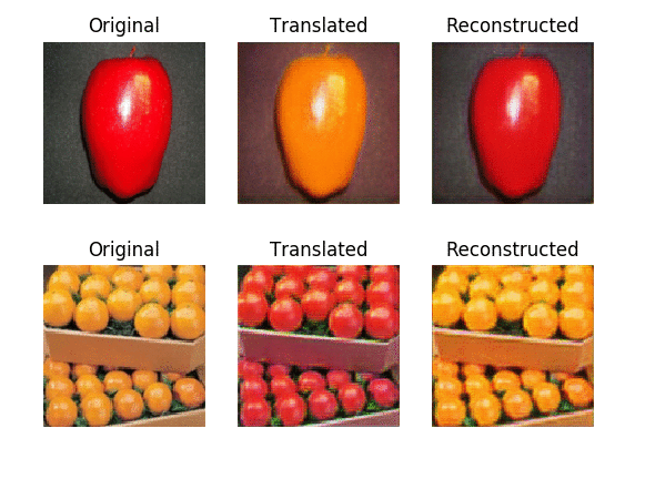
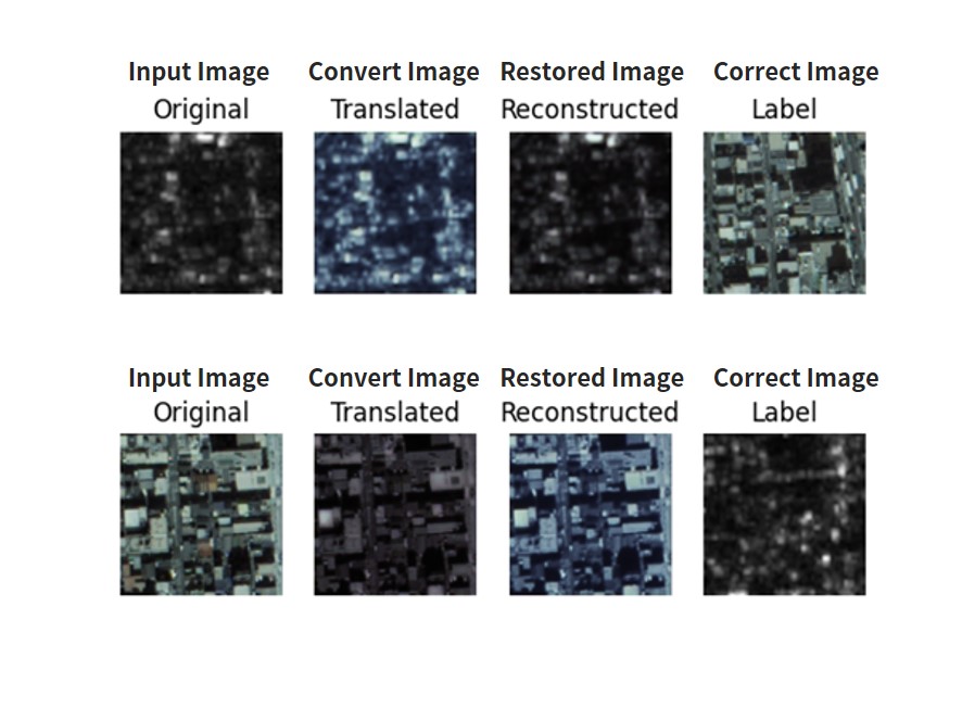
The learning process will also save every 200 times in a folder called images. The results of the learning for 200 times and 3000 times are as follows.
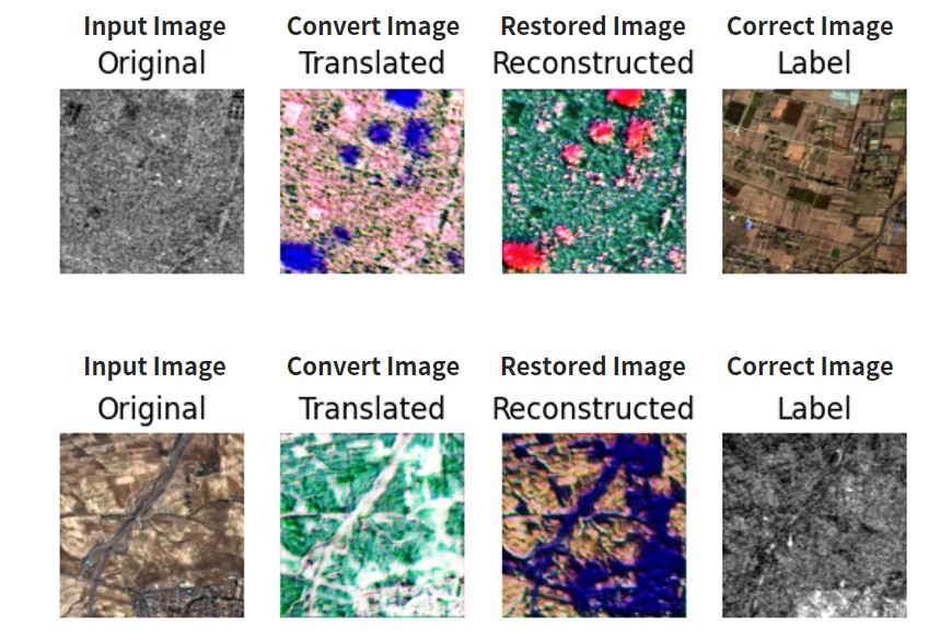
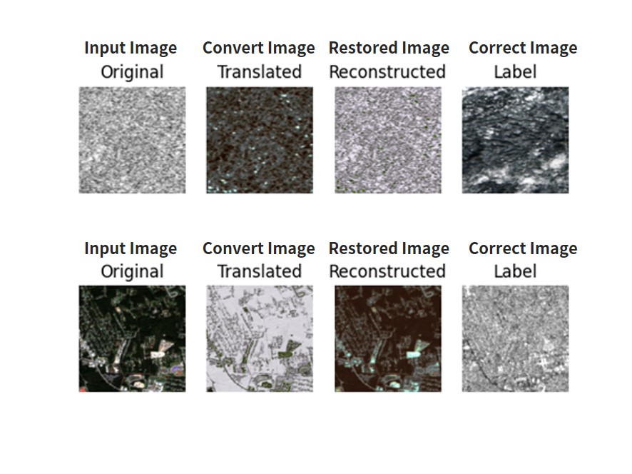
“Original” is the inputed image, “Translated” is the converted image, “Reconstructed” is the original image that has been reconstructed, and “Label” is the final data. In other words, Original+Reconstructed, and Translated+Label both have to perfectly match each other. If you write it in the formula we explained in the beginning, it should look like the following.
Original: x *horse
Translated: y := f(x) *zebra
Reconstructed: x := g(f(x)) *horse
Label: y *zebra
The upper part is the image converted as SAR→optical→SAR. The lower part is the image converted as optical→SAR→optical.
When you compare the learning when it has been conducted 200 and 3000 times, you can see that it is gradually getting closer to the SAR image. The learning that has been done 200 times is still rough around the edges, but after 3000 times you can see it getting pretty close to a SAR image. These results are very interesting because they are close to what you would get if you had a matching pair, even though we just ran the learning on the two different images with brute force.
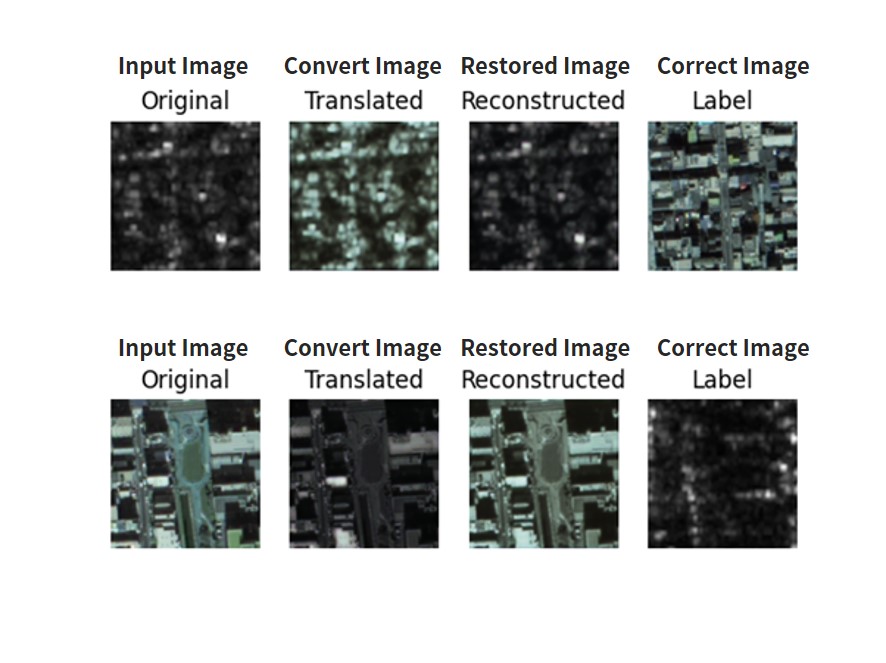
Here are the results of some images we ran the learning on.
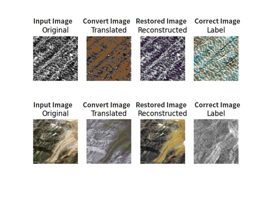
Converting a SAR image into an optical image requires up-sampling from less data to more data, meaning the opposite won’t come out as clean.
*Up-sampling: A process that adds to the original data, increasing its pixels by 2 times.
4.2. ASNARO-1 (optical image) and ALOS-2 (SAR image) Data
Next we will be running the program with the following data set. First, we will split the 2 images we created earlier so that they can be used as data sets. Run in the following program in the folder where we ran cyclegan.py earlier.
import cv2
import os
import random
import copy as cp
generation_size = 256
generation_num = 1000
img_a = cv2.imread("SAR.png")
img_b = cv2.imread("OPTICAL.png")
limit_y = img_a.shape[0] - generation_size
output_dir = "./datasets/customsar/"
os.makedirs( output_dir + 'trainA', exist_ok=True)
os.makedirs( output_dir + 'trainB', exist_ok=True)
os.makedirs( output_dir + 'testA', exist_ok=True)
os.makedirs( output_dir + 'testB', exist_ok=True)

for i in range(generation_num):
  offset_y = random.randint(generation_size, img_a.shape[0]) - generation_size
  offset_x = random.randint(generation_size, img_a.shape[1]) - generation_size
  new_a = cp.deepcopy(img_a[offset_y:offset_y+generation_size, offset_x:offset_x+generation_size, :])
  new_b = cp.deepcopy(img_b[offset_y:offset_y+generation_size, offset_x:offset_x+generation_size, :])
  cv2.imwrite(output_dir + "trainA/" + str(i) + ".png", new_a)
  cv2.imwrite(output_dir + "trainB/" + str(i) + ".png", new_b)

split_num = int(img_a.shape[1] / generation_size)
for i in range(split_num):
  offset_y = img_a.shape[0] - generation_size
  offset_x = i * generation_size
  new_a = cp.deepcopy(img_a[offset_y:offset_y+generation_size, offset_x:offset_x+generation_size, :])
  new_b = cp.deepcopy(img_b[offset_y:offset_y+generation_size, offset_x:offset_x+generation_size, :])
  cv2.imwrite(output_dir + "testA/" + str(i) + ".png", new_a)
  cv2.imwrite(output_dir + "testB/" + str(i) + ".png", new_b)
If you run this, it will create the folders “trainA, trainB, testA, testB” in eth the ./datasets/customar/ folder array, splitting up images for each domain for you. A is the SAR domain, and B is the optical domain.
Next, we will make changes to the cyclegan.py as follows and run it again.
pre-change self.dataset_name = ‘sar’
post-change self.dataset_name = ‘customsar’
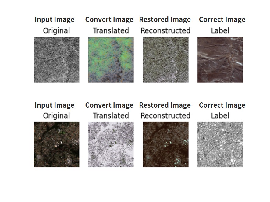
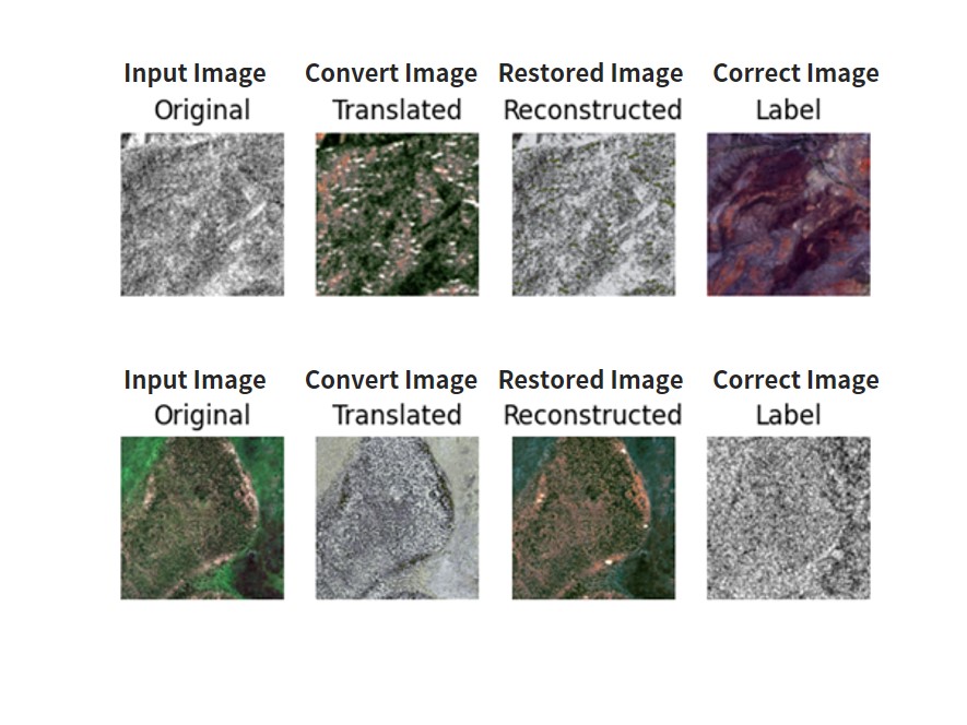
It should give you this after you run it.
While it wasn’t converted as well as our other data set and its resolution is lower, it has given us a similar image. The parts of the SAR images that were likely to reflect have been left white, with the rest of the image learning to become darker.
Since both the Sentinel-1/2 and ASNARO-1/ALOS-2 pairs are learned randomly, the ASNARO-1/ALOS-2 data set also has a higher resolution for its SAR images, making the quality about the same as our first data set.
Let’s try testing it out on a few other images.

5. Converting Between Optical↔SAR Images With Supervised Learning (pix2pix)
Let’s see what happens when we used supervised data to learn. Just like we did for CycleGAN, you can find what you need here: https://github.com/eriklindernoren/Keras-GAN/tree/master/pix2pix Changes have been made mainly about version compatibility, data loader, etc. We are using the same data set we used for CycleGAN, so let’s copy these data sets to a different folder where we will run our progam. Our new folder will act as our route directory. If you follow the instructions and run the program it should create the following folders.
root
|- pix2pix.py
|- data_loader_py
|- datasets
| |- sat
| |-testA
| | |- file...
| |-testB
| | |- file...
| |-trainA
| | |- file...
| |-trainB
| |- file...
|- images
|- sar
|- file…
5.1. High-Quality Optical and SAR Image Pairs (Sentinel-1, 2)
First, it will show you the data loaded by the data loader. Save with the name “data_loader.py”.
import scipy
from glob import glob
import numpy as np
import matplotlib.pyplot as plt

class DataLoader():
    def __init__(self, dataset_name, img_res=(128, 128)):
        self.dataset_name = dataset_name
        self.img_res = img_res

    def load_data(self, batch_size=1, is_testing=False):
        data_type = "train" if not is_testing else "test"
        path = glob('./datasets/%s/%s/*' % (self.dataset_name, data_type))

        batch_images = np.random.choice(path, size=batch_size)

        imgs_A = []
        imgs_B = []
        for img_path in batch_images:
            img = self.imread(img_path)

            h, w, _ = img.shape
            _w = int(w/2)
            img_A, img_B = img[:, :_w, :], img[:, _w:, :]

            img_A = scipy.misc.imresize(img_A, self.img_res)
            img_B = scipy.misc.imresize(img_B, self.img_res)

            # If training => do random flip
            if not is_testing and np.random.random()  0.5:
                        img_A = np.fliplr(img_A)
                        img_B = np.fliplr(img_B)

                imgs_A.append(img_A)
                imgs_B.append(img_B)

            imgs_A = np.array(imgs_A)/127.5 - 1.
            imgs_B = np.array(imgs_B)/127.5 - 1.

            yield imgs_A, imgs_B

    def load_data_with_label_batch(self, domain, batch_size=1, is_testing=False):
        data_type = "train%s" % domain if not is_testing else "test%s" % domain
        path = glob('./datasets/%s/%s/*' % (self.dataset_name, data_type))
        batch_images = np.random.choice(path, size=batch_size)
        imgs = []
        lbls = []
        for img_path in batch_images:
            img = self.imread(img_path)
            # lbl path
            if "A/" in img_path:
              lbl_path = img_path.replace('s1_', 's2_')
              lbl_path = lbl_path.replace('A/', 'B/')
            else:
              lbl_path = img_path.replace('s2_', 's1_')
              lbl_path = lbl_path.replace('B/', 'A/')
            lbl = self.imread(lbl_path)

            if not is_testing:
                img = scipy.misc.imresize(img, self.img_res)
                lbl = scipy.misc.imresize(lbl, self.img_res)

                if np.random.random() > 0.5:
                    img = np.fliplr(img)
                    lbl = np.fliplr(lbl)
            else:
                img = scipy.misc.imresize(img, self.img_res)
                lbl = scipy.misc.imresize(lbl, self.img_res)
            imgs.append(img)
            lbls.append(lbl)
        imgs = np.array(imgs)/127.5 - 1.
        lbls = np.array(lbls)/127.5 - 1.
        return imgs, lbls


    def imread(self, path):
        return scipy.misc.imread(path, mode='RGB').astype(np.float)
Next is the program you need to use on Pix2Pix. Save it with the name “pix2pix.py”.
from __future__ import print_function, division
import scipy
from keras.datasets import mnist
from keras_contrib.layers.normalization.instancenormalization import InstanceNormalization
from keras.layers import Input, Dense, Reshape, Flatten, Dropout, Concatenate
from keras.layers import BatchNormalization, Activation, ZeroPadding2D
from keras.layers.advanced_activations import LeakyReLU
from keras.layers.convolutional import UpSampling2D, Conv2D
from keras.models import Sequential, Model
from tensorflow.keras.optimizers import Adam
import datetime
import matplotlib.pyplot as plt
import sys
from data_loader import DataLoader
import numpy as np
import os
import matplotlib as mpl
mpl.use('Agg')
import matplotlib.pyplot as plt

class Pix2Pix():
    def __init__(self):
        # Input shape
        self.img_rows = 256
        self.img_cols = 256
        self.channels = 3
        self.img_shape = (self.img_rows, self.img_cols, self.channels)

        # Configure data loader
        self.dataset_name = 'sar'
        self.data_loader = DataLoader(dataset_name=self.dataset_name,
                                      img_res=(self.img_rows, self.img_cols))


        # Calculate output shape of D (PatchGAN)
        patch = int(self.img_rows / 2**4)
        self.disc_patch = (patch, patch, 1)

        # Number of filters in the first layer of G and D
        self.gf = 64
        self.df = 64

        optimizer = Adam(0.0002, 0.5)

        # Build and compile the discriminator
        self.discriminator = self.build_discriminator()
        self.discriminator.compile(loss='mse',
            optimizer=optimizer,
            metrics=['accuracy'])

        #-------------------------
        # Construct Computational
        #   Graph of Generator
        #-------------------------

        # Build the generator
        self.generator = self.build_generator()

        # Input images and their conditioning images
        img_A = Input(shape=self.img_shape)
        img_B = Input(shape=self.img_shape)

        # By conditioning on B generate a fake version of A
        fake_A = self.generator(img_B)

        # For the combined model we will only train the generator
        self.discriminator.trainable = False

        # Discriminators determines validity of translated images / condition pairs
        valid = self.discriminator([fake_A, img_B])

        self.combined = Model(inputs=[img_A, img_B], outputs=[valid, fake_A])
        self.combined.compile(loss=['mse', 'mae'],
                              loss_weights=[1, 100],
                              optimizer=optimizer)

    def build_generator(self):
        """U-Net Generator"""

        def conv2d(layer_input, filters, f_size=4, bn=True):
            """Layers used during downsampling"""
            d = Conv2D(filters, kernel_size=f_size, strides=2, padding='same')(layer_input)
            d = LeakyReLU(alpha=0.2)(d)
            if bn:
                d = BatchNormalization(momentum=0.8)(d)
            return d

        def deconv2d(layer_input, skip_input, filters, f_size=4, dropout_rate=0):
            """Layers used during upsampling"""
            u = UpSampling2D(size=2)(layer_input)
            u = Conv2D(filters, kernel_size=f_size, strides=1, padding='same', activation='relu')(u)
            if dropout_rate:
                u = Dropout(dropout_rate)(u)
            u = BatchNormalization(momentum=0.8)(u)
            u = Concatenate()([u, skip_input])
            return u

        # Image input
        d0 = Input(shape=self.img_shape)

        # Downsampling
        d1 = conv2d(d0, self.gf, bn=False)
        d2 = conv2d(d1, self.gf*2)
        d3 = conv2d(d2, self.gf*4)
        d4 = conv2d(d3, self.gf*8)
        d5 = conv2d(d4, self.gf*8)
        d6 = conv2d(d5, self.gf*8)
        d7 = conv2d(d6, self.gf*8)

        # Upsampling
        u1 = deconv2d(d7, d6, self.gf*8)
        u2 = deconv2d(u1, d5, self.gf*8)
        u3 = deconv2d(u2, d4, self.gf*8)
        u4 = deconv2d(u3, d3, self.gf*4)
        u5 = deconv2d(u4, d2, self.gf*2)
        u6 = deconv2d(u5, d1, self.gf)

        u7 = UpSampling2D(size=2)(u6)
        output_img = Conv2D(self.channels, kernel_size=4, strides=1, padding='same', activation='tanh')(u7)

        return Model(d0, output_img)

    def build_discriminator(self):

        def d_layer(layer_input, filters, f_size=4, bn=True):
            """Discriminator layer"""
            d = Conv2D(filters, kernel_size=f_size, strides=2, padding='same')(layer_input)
            d = LeakyReLU(alpha=0.2)(d)
            if bn:
                d = BatchNormalization(momentum=0.8)(d)
            return d

        img_A = Input(shape=self.img_shape)
        img_B = Input(shape=self.img_shape)

        # Concatenate image and conditioning image by channels to produce input
        combined_imgs = Concatenate(axis=-1)([img_A, img_B])

        d1 = d_layer(combined_imgs, self.df, bn=False)
        d2 = d_layer(d1, self.df*2)
        d3 = d_layer(d2, self.df*4)
        d4 = d_layer(d3, self.df*8)

        validity = Conv2D(1, kernel_size=4, strides=1, padding='same')(d4)

        return Model([img_A, img_B], validity)

    def train(self, epochs, batch_size=1, sample_interval=50):

        start_time = datetime.datetime.now()

        # Adversarial loss ground truths
        valid = np.ones((batch_size,) + self.disc_patch)
        fake = np.zeros((batch_size,) + self.disc_patch)

        for epoch in range(epochs):
            for batch_i, (imgs_A, imgs_B) in enumerate(self.data_loader.load_batch(domain="A", batch_size=batch_size)):

                # ---------------------
                #  Train Discriminator
                # ---------------------

                # Condition on B and generate a translated version
                fake_A = self.generator.predict(imgs_B)

                # Train the discriminators (original images = real / generated = Fake)
                d_loss_real = self.discriminator.train_on_batch([imgs_A, imgs_B], valid)
                d_loss_fake = self.discriminator.train_on_batch([fake_A, imgs_B], fake)
                d_loss = 0.5 * np.add(d_loss_real, d_loss_fake)

                # -----------------
                #  Train Generator
                # -----------------

                # Train the generators
                g_loss = self.combined.train_on_batch([imgs_A, imgs_B], [valid, imgs_A])

                elapsed_time = datetime.datetime.now() - start_time
                # Plot the progress
                print ("[Epoch %d/%d] [Batch %d/%d] [D loss: %f, acc: %3d%%] [G loss: %f] time: %s" % (epoch, epochs,
                                                                        batch_i, self.data_loader.n_batches,
                                                                        d_loss[0], 100*d_loss[1],
                                                                        g_loss[0],
                                                                        elapsed_time))

                # If at save interval => save generated image samples
                if batch_i % sample_interval == 0:
                    self.sample_images(epoch, batch_i)

    def sample_images(self, epoch, batch_i):
        os.makedirs('images/%s' % self.dataset_name, exist_ok=True)
        r, c = 3, 3

        imgs_A, imgs_B = self.data_loader.load_data_with_label_batch(domain="A", batch_size=3, is_testing=True)
        fake_A = self.generator.predict(imgs_B)

        gen_imgs = np.concatenate([imgs_B, fake_A, imgs_A])

        # Rescale images 0 - 1
        gen_imgs = 0.5 * gen_imgs + 0.5

        titles = ['Condition', 'Generated', 'Original']
        fig, axs = plt.subplots(r, c)
        cnt = 0
        for i in range(r):
            for j in range(c):
                axs[i,j].imshow(gen_imgs[cnt])
                axs[i, j].set_title(titles[i])
                axs[i,j].axis('off')
                cnt += 1
        fig.savefig("images/%s/%d_%d.png" % (self.dataset_name, epoch, batch_i))
        plt.close()


if __name__ == '__main__':
    gan = Pix2Pix()
    gan.train(epochs=200, batch_size=3, sample_interval=200)
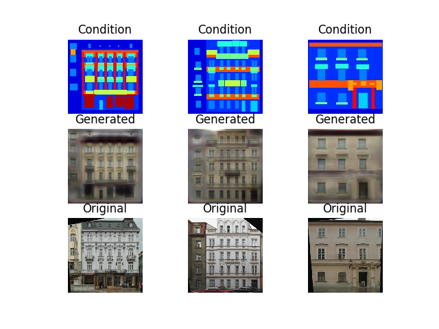
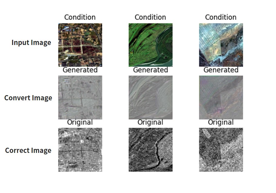
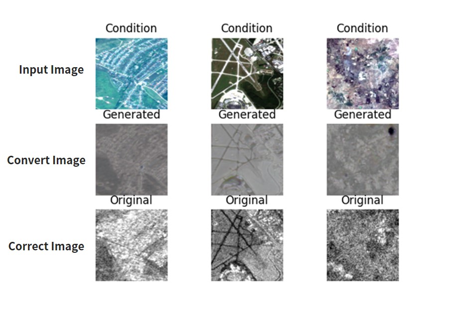
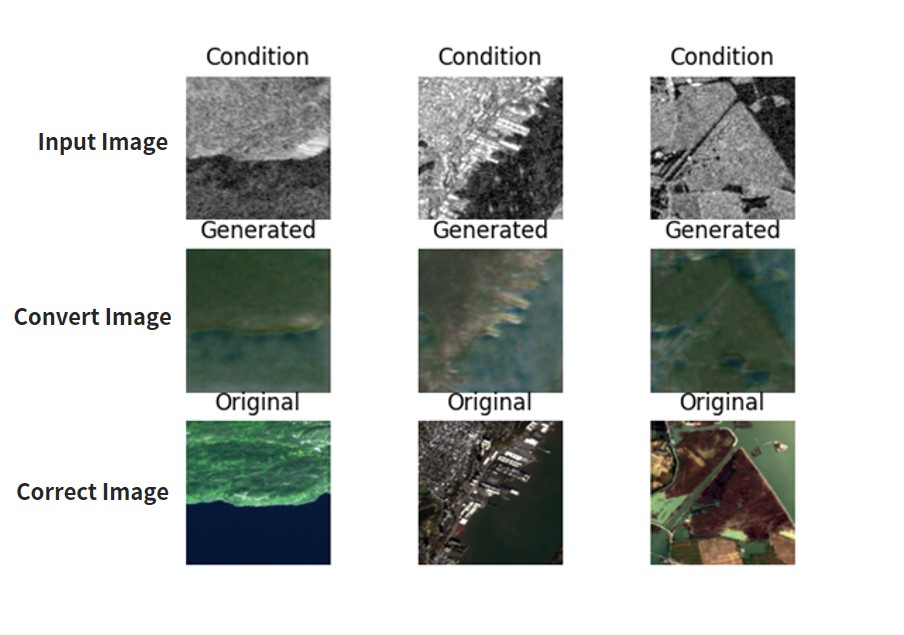
Performing this code gives you the following.
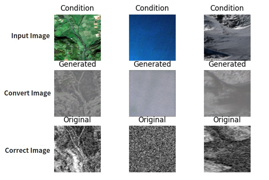
“Condition” is the input image (optical image), “Generated” is the converted image (SAR image), and “Original” is the final (SAR image). We want “Generated” and “Original” to match up.
It feels like supervised learning gives us a more accurate image, but not by much. Here are a few more examples.
Furthermore, to learn how to convert from SAR to optical images, change the following and let it learn.
pre-change for batch_i, (imgs_A, imgs_B) in
enumerate(self.data_loader.load_batch(domain=”A”, batch_size=batch_size)):
post-change for batch_i, (imgs_A, imgs_B) in
enumerate(self.data_loader.load_batch(domain=”B”, batch_size=batch_size)):
pre-change imgs_A, imgs_B =
self.data_loader.load_data_with_label_batch(domain=”A”, batch_size=3, is_testing=True)
post-change imgs_A, imgs_B =
self.data_loader.load_data_with_label_batch(domain=”B”, batch_size=3, is_testing=True)
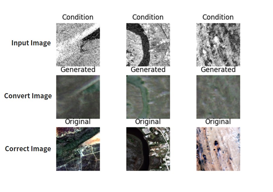
Running it should give you the following results.
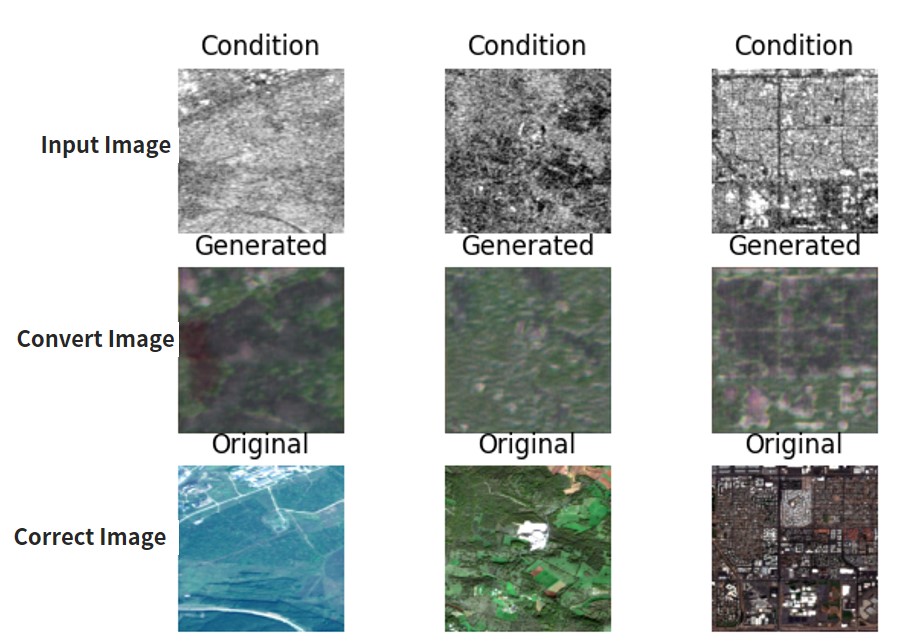
It looks like we get better results converting optical to SAR then SAR to optical. This is interesting because optical seems to require more data. But it looks like it tends to mess up the colors. Here are other examples.
5.2. ASNARO-1 (optical image) and ALOS-2 (SAR image) Data
As with unsupervised learning, only the following parts should be changed and executed.
pre-change self.dataset_name = ‘sar’
post-change self.dataset_name = ‘customsar’
*To convert optical to SAR, revert the domain in the source code that we mentioned earlier to its original form.
You should get the following results.
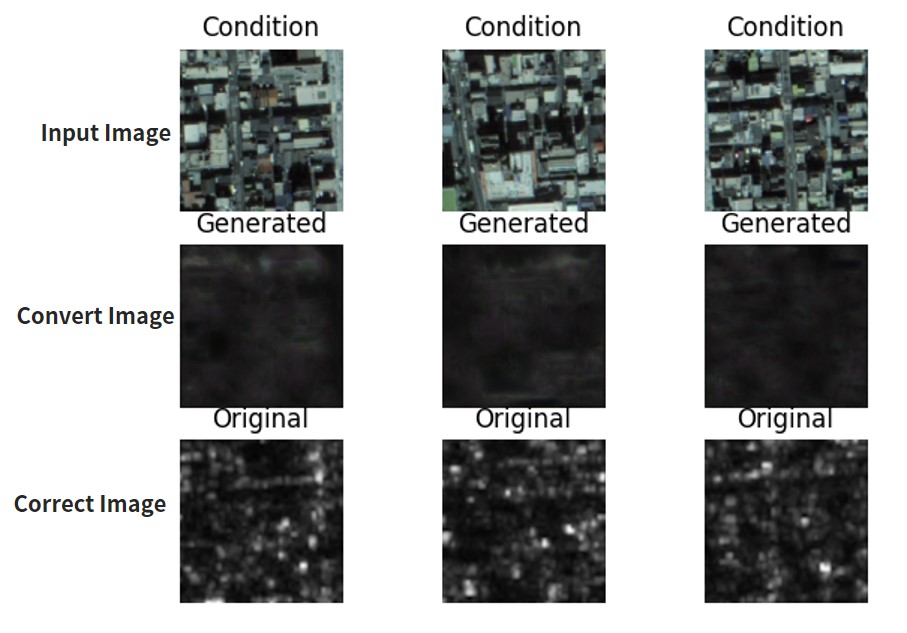
SInce the quality isn’t as high for these pairs (the resolution, conditions, observational period, etc. aren’t the same), the results aren’t that great either. The other results have also come back almost entirely black. So as you can see, unsupervised learning with CycleGAN seems to produce better results. The results, of course, will vary depending on how much you have the machine learn, so please try it for yourself.
Next, let’s try converting SAR to optical. The method is the same as in the other data set. We have to change the source code for pix2pix.py done as follows.
pre-change for batch_i, (imgs_A, imgs_B) in
enumerate(self.data_loader.load_batch(domain=”A”, batch_size=batch_size)):
post-change
for batch_i, (imgs_A, imgs_B) in enumerate(self.data_loader.load_batch(domain=”B”, batch_size=batch_size)):
pre-change imgs_A, imgs_B =
self.data_loader.load_data_with_label_batch(domain=”A”, batch_size=3, is_testing=True)
post-change imgs_A, imgs_B =
self.data_loader.load_data_with_label_batch(domain=”B”, batch_size=3, is_testing=True)
Performing this code gives you the following.
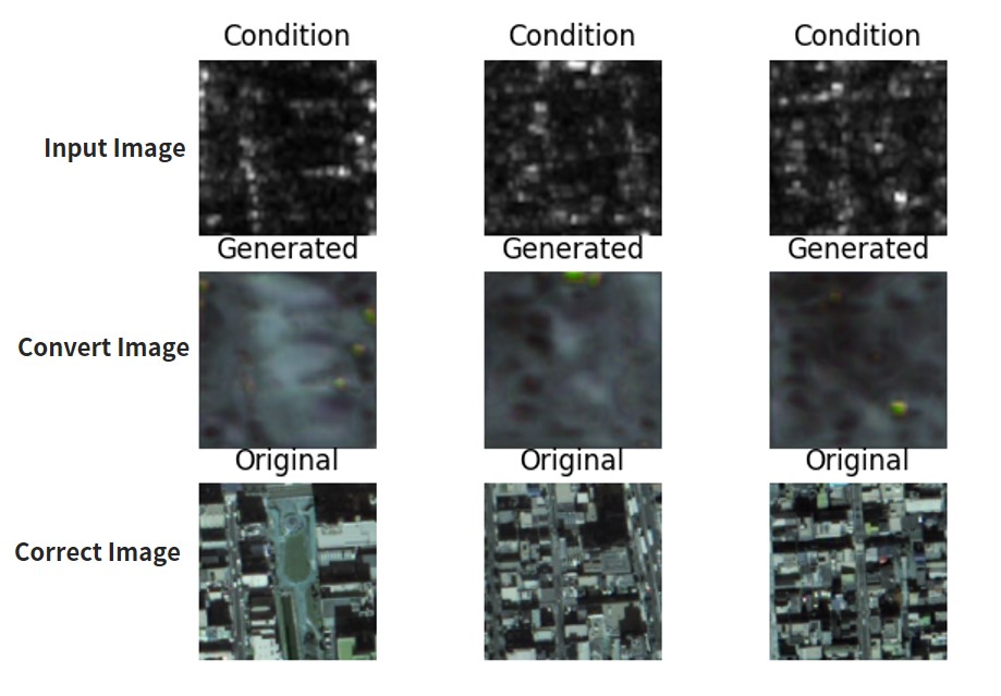
Almost none of these were able to convert accurately. The rest of the results came back blurry as well. The quality of the results of supervised learning depend heavily on the quality of the images.
That brings us to the end of our article. Today we used two pairs of images; ASNARO-1 and ALOS-2, and Sentinel-1 and Sentinel-2, to test out unsupervised learning (cycleGAN) and supervised learning (Pix2Pix) for converting SAR and optical images into each other. For our summary, I’d like create a matrix that shows where each of the combinations excel.
6. Summary
In this article, we tried the following:
– Collect a rough batch of ASNARO-1 (an optical satellite) and ALOS-2 (an SAR satellite) data, and convert between optical↔SAR images.
– Use a somewhat high-quality optical/SAR image pair (Sentinel-1, 2) to convert between optical↔SAR images.
– Compare the difference between supervised (Pix2Pix) and unsupervised (CycleGAN) learning to convert between optical↔SAR images.
We used two methods and two sets for a total of four combinations Here is a comparison of the four combinations.
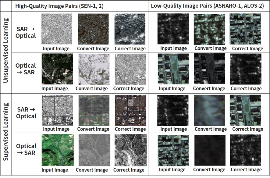
When you have high-quality data, it works well for both supervised and unsupervised images. When you have low-quality data, the unsupervised data is able to convert it to a certain extent, but supervised data couldn’t convert at all. You can see our comparison in the matrix below.
| High-Quality Image Pairs (Sentinel-1, 2) | Low-Quality Image Pairs (ASNARO-1, ALOS-2) | |
| Unsupervised Learning | 〇 | 〇 |
| Supervised Learning | 〇 | × |
In conclusion, if you don’t have access to high-quality data, it is better to use CycleGAN to use unsupervised data. If you have access to high-quality data, however, there isn’t a big difference between using supervised or unsupervised data.
We also learned that you can use unsupervised data to create SAR images even when you don’t have optimal data. By using this technique, you can tell what images taken by an optical satellite looked like if it had a SAR sensor or the other way around. You can also run a simulation to see what objects that have never been taken with SAR look like. This method can be used in a wide variety of ways, so try it out for yourself.
Thanks for reading!