Structural Classifications Using SAR Polarimetry (Polarimetric Decomposition)
In today's article, we will be testing out whether or not you can use polarimetric decomposition to differentiate between natural and man-made objects.
We have introduced a few different concepts about SAR, the satellite observation technology, here on Sorabatake.
The use of SAR technology is seeing a significant increase thanks to it allowing us to actively observe the earth using electromagnetic waves, which aren’t affected by poor weather conditions such as rain and clouds.
That being said, when you actually look at SAR images, they are different from normal images in that they are in black and white, and very grainy, which likely turns off a lot of people to them.
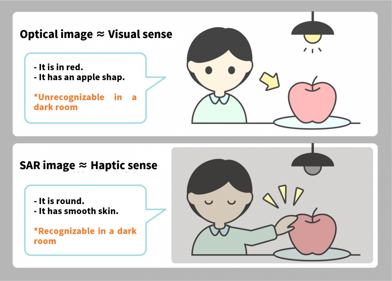
Optical images are to SAR images as sight is to touch.
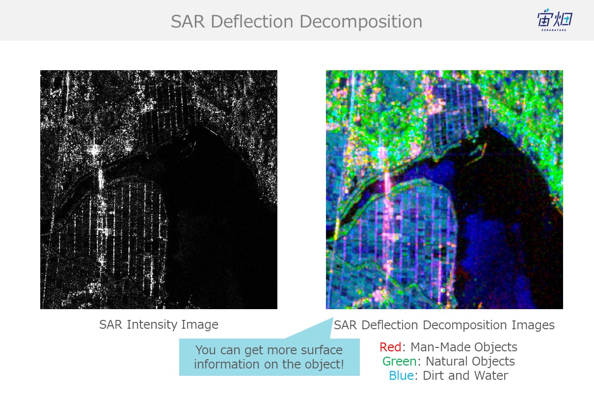
SAR images may seem like just black and white images, but they contain information on surface texture and more, which is extractable if you know what you are doing.
The process of extracting such information is called polarimetric decomposition.
Polarimetric decomposition is useful for accurately identifying different textures on the earth’s surface.
This process is not only useful for differentiating between natural and man-made objects, but it could also help with handling SAR images.
There are lots of ways to get rid of noise to make SAR images easier to handle, but the approach we take in this article allows us to add new information to the entire photo, making it a very effective way to prep them.
This prep technique will be increasingly important to know as SAR imagery grows more common, so please stay with us as we get into some finer details.
In this article, we will use polarimetric decomposition to test whether or not we can tell the difference between man-made and natural objects on Tellus.
Detecting Texture Using "Polarimetric Decomposition"
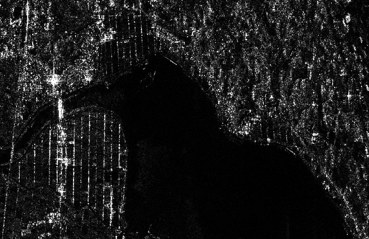
Black and White SAR Images are "Intensity Images"

Most people probably associate SAR with black and white images.
This is because electromagnetic waves use black and white to convey the intensity of whatever they have reflected off of.
The right side is water, and due to specular reflection, most electromagnetic waves aimed at water diverge off into another direction away from the satellite resulting in it showing up pitch-black in SAR images. The left side is full of man-made objects which are better at reflecting waves back to the satellite. You can see how objects on the right show up brighter, which means they are more intense.
Behaviour of Electromagnetic Waves: Scattering and Reflection
Let’s define scattering and reflection.
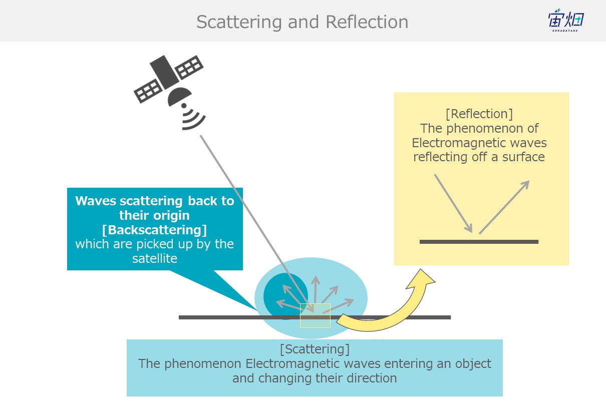
Scattering occurs when the energy from electromagnetic waves that have entered an object partially convert into new electromagnetic waves that disperse from that object in multiple different directions.
When waves enter an object with different electrical properties, scattering causes different phenomena such as reflection and refraction.
Reflection is simply the reflection of electromagnetic waves.
When waves reflect off of objects back in the direction they originated, it is called backscattering. SAR images use backscattered electromagnetic waves to create images.
Different Backscattering Processes for SAR -- Specular Reflection, Corner Reflection, Surface Scattering, and Volume Scattering --
Let’s breakdown the behaviour of electromagnetic waves emitted by satellites.
The way they reflect, or the process with which they scatter off of objects that waves come into contact varies. The following are four behaviours often exhibited by waves.
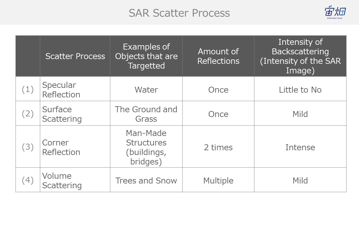
We can gather the number of reflections and level of backscattering (which equate to intensity for SAR images) from SAR images to identify the objects they capture.
That being said, the specular reflection that occurs for (1) sees little to no backscattering, which means we won’t be able to identify it using polarimetric analysis this time.
We explain each of the processes below.
(1) Specular Reflection (for flat, smooth surfaces such as water)
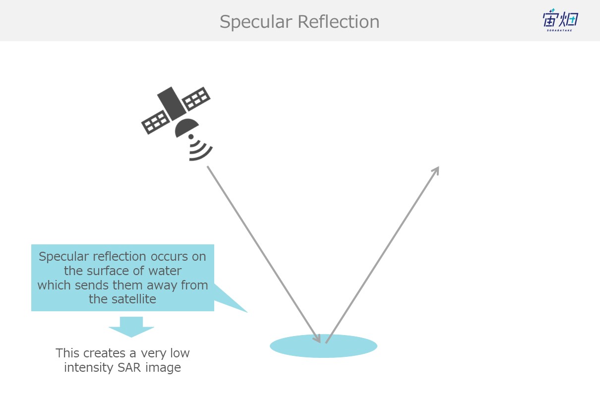
Waves undergo specular reflection when they hit smooth wet surfaces like water, which results in little to no waves making it back to the satellite. This causes dark spots (due to low intensity) to show up in the images.
This is referred to as single scattering.
(2) Surface Scattering (the earth's surface, grass, etc.)
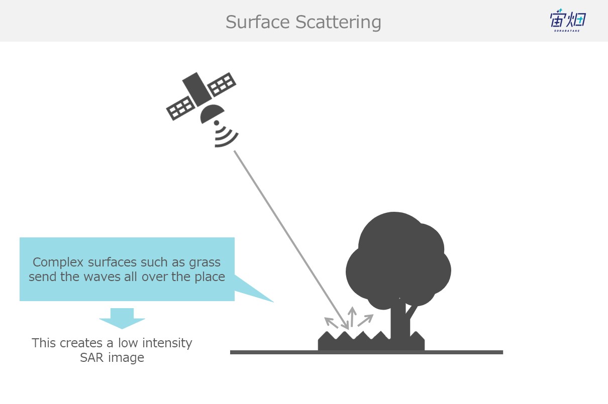
When waves reflect off of the ground (grass, etc.) they get sent off into all different directions. This is called surface scattering. Waves that undergo surface scattering only partially make it back to the satellite, resulting in a lower intensity.
This is also known as a single reflection.
(3) Corner Reflection (man-made objects such as buildings, bridges, etc.)
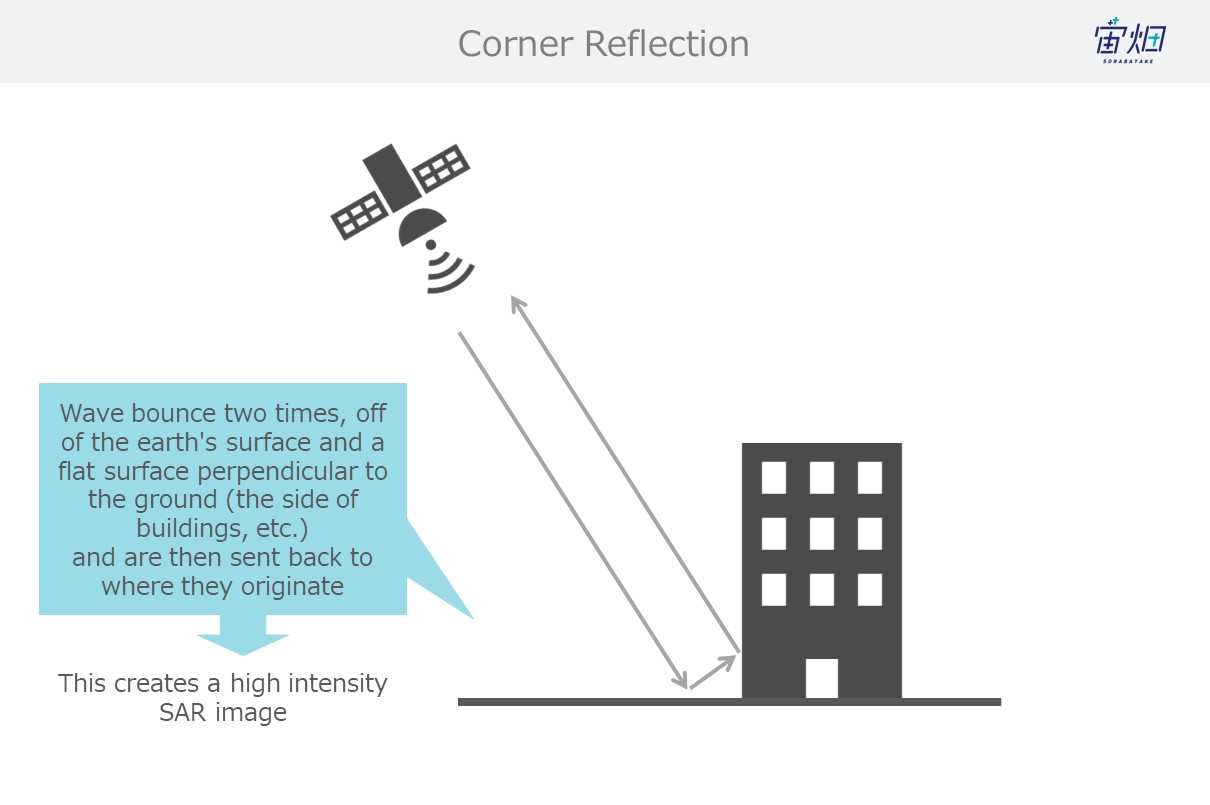
Buildings and other objects with flat surfaces that are built perpendicular from the earth’s surface capture waves that bounce off the earth’s surface and send them back to the satellite. This is called double reflection.
Most of the radio waves that follow this path make it back to the satellite, resulting in a more intense signal.
(4) Trees, Snow, Etc. (volume scattering)
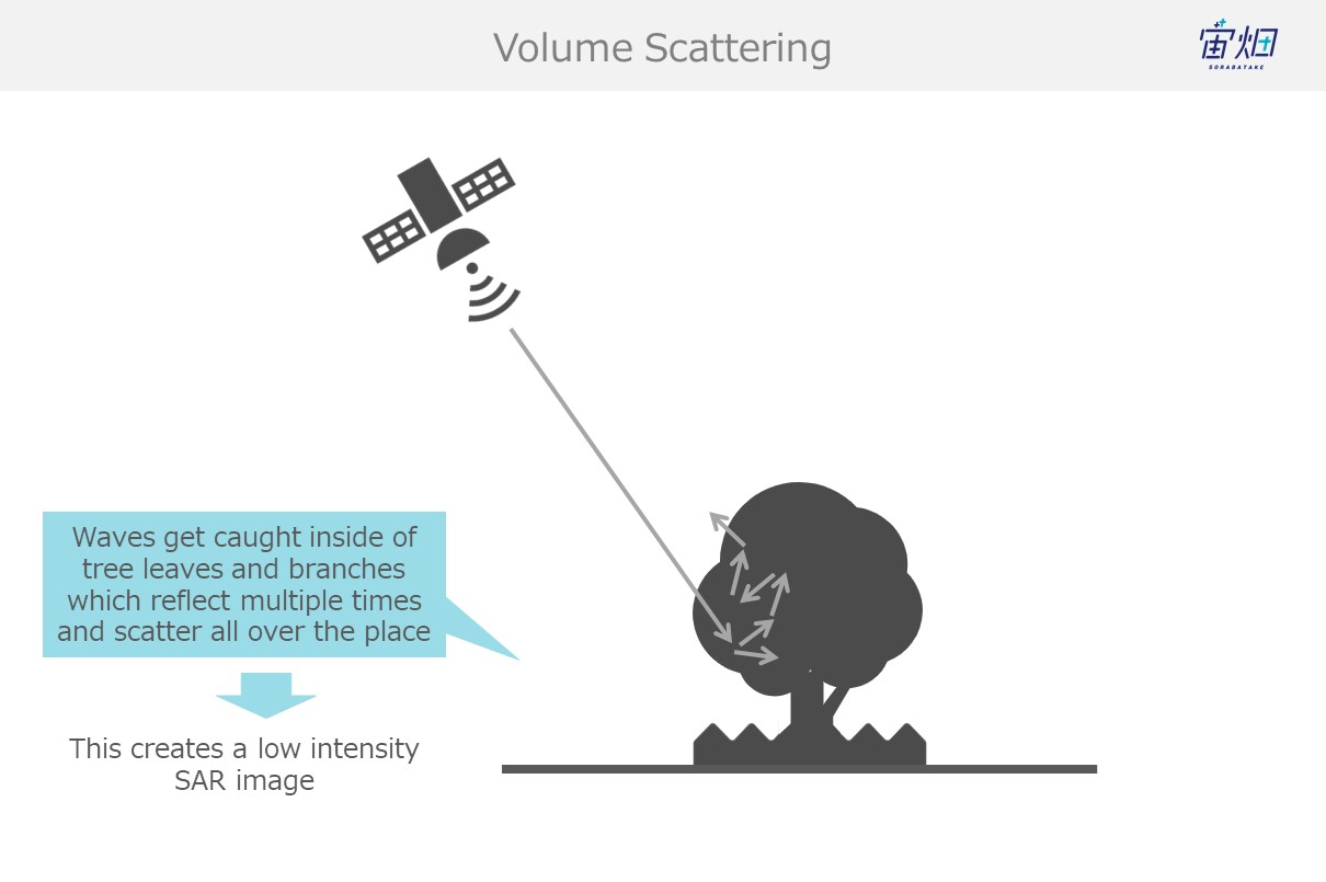
Waves that find their way into trees get caught up in their leaves and branches, resulting in a chain of reflections (volume scattering) that results in most waves not making their way back to the satellite and a low intensity image. This phenomenon is seen often with trees and snow.
The big difference between surface scattering and volume scattering is the number of times the waves are reflected. Waves that undergo surface scattering only reflect off of one object, but volume scattering involves being reflected multiple times.
Classifying Blurriness and Glare With Polarimetry
These different examples of reflection and scattering that we have introduced can be classified by using polarimetry specific to SAR observation.
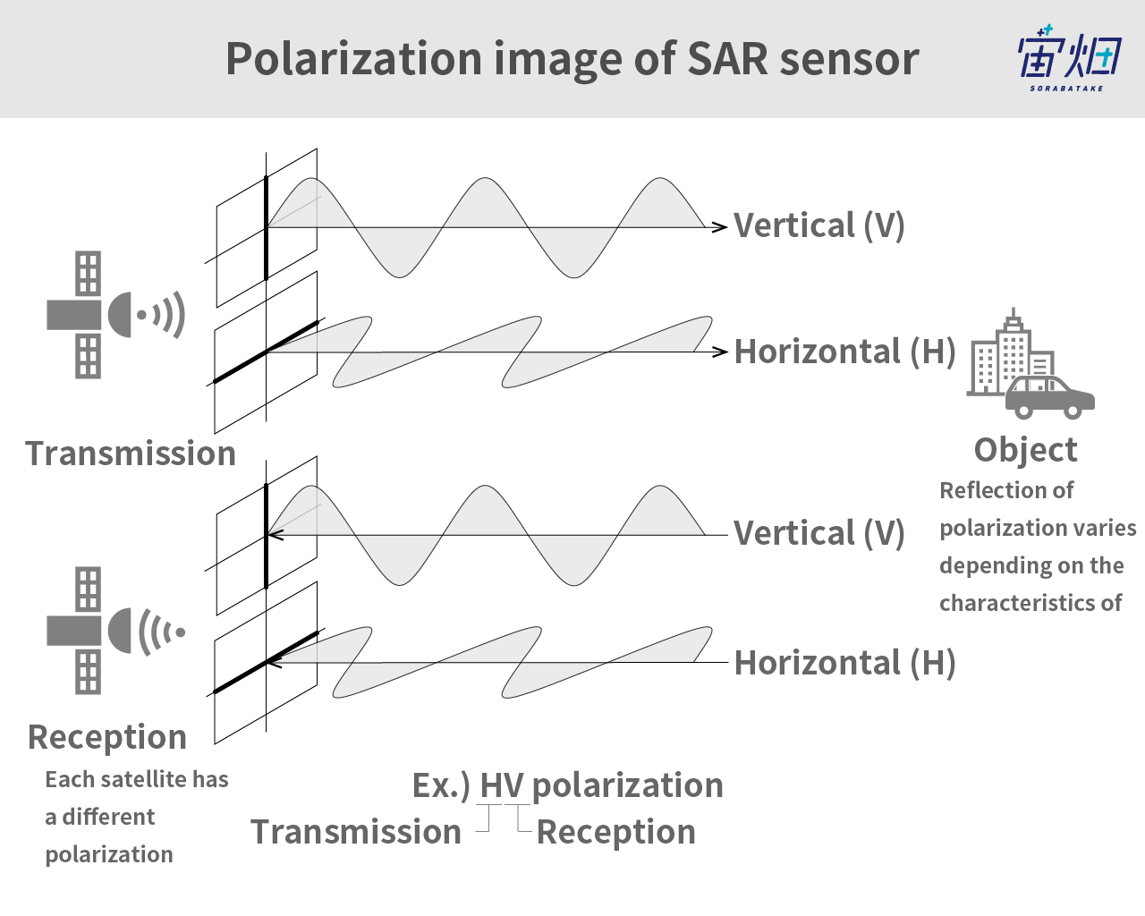
Electromagnetic waves emitted by SAR sensors can be broken down into horizontal and vertical components of polarimetry, which oscillate in different directions, as shown in the figure above.
By emitting horizontal polarimetry (H) and vertical polarimetry (V), the waves that come back to the satellite are also horizontal (H) and vertical (V).
The combination of a horizontal emission and horizontal reception is HH, horizontal emission and vertical reception is HV, vertical emission and vertical reception is VV, and vertical emission and horizontal reception is VH. Some larger satellites can receive microwaves both horizontally and vertically at the same time. This feature is called, for instance, HH-HV.
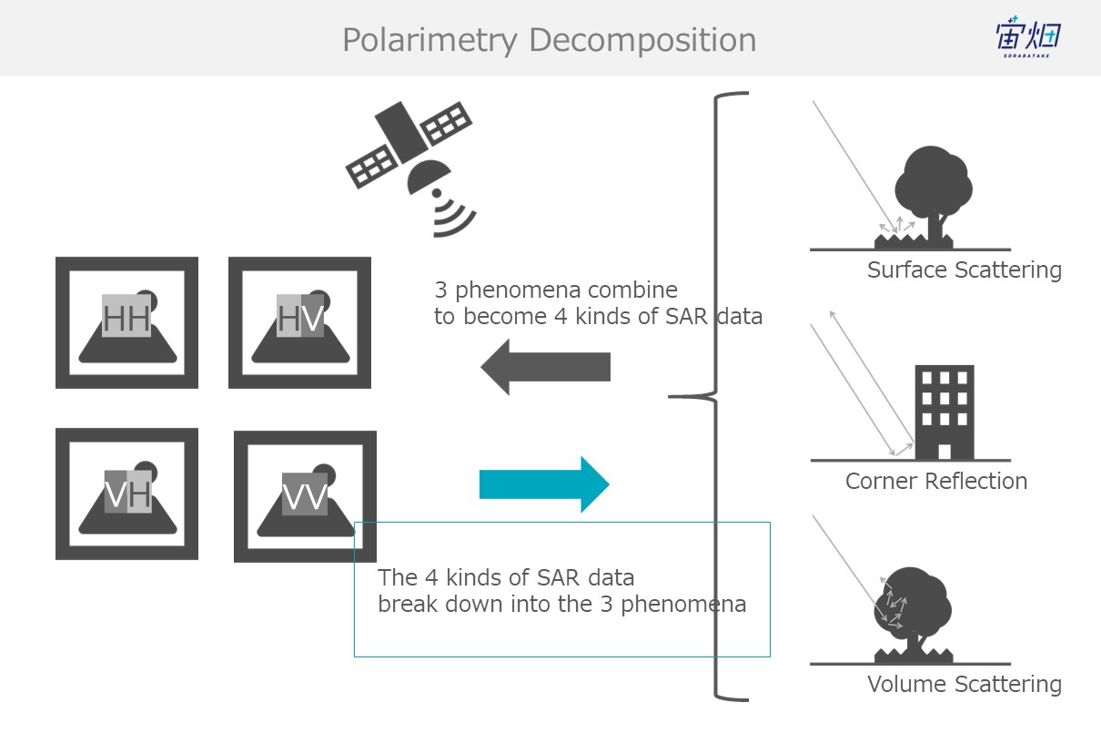
The components that make up polarized waves depend on their scattering behaviour (surface scattering, corner reflection, and volume scattering). This allows us to detect the polarimetry (of the 4 polarized waves) of the SAR images, and classify their scatter process as single reflection (surface scattering), double reflection, or volume scattering. This is called “polarimetric decomposition”.
Attaining Polarimetry CEOS
In order to perform polarimetric decomposition, we need data for each of the four different kinds of waves. We will use polarimetry data from the following article as a reference.
Imaging PALSAR-2 L1.1 using Tellus [with code]
import os, requests
import geocoder # ! pip install geocoder

# Fields
BASE_API_URL = "https://file.tellusxdp.com/api/v1/origin/search/" # https://www.tellusxdp.com/docs/api-reference/palsar2-files-v1.html#/
ACCESS_TOKEN = "YOUR_TOKEN"
HEADERS = {"Authorization": "Bearer " + ACCESS_TOKEN}
TARGET_PLACE="kasumigaura, ibaraki"
SAVE_DIRECTORY="./data/"

# Functions
def rect_vs_point(ax, ay, aw, ah, bx, by):
    return 1 if bx > ax and bx  ay and by < ah else 0
def get_scene_list_slc(_get_params={}):
    query = "palsar2-l11"
    r = requests.get(BASE_API_URL + query, _get_params, headers=HEADERS)
    if not r.status_code == requests.codes.ok:
        r.raise_for_status()
    return r.json()

def get_slc_scenes(_target_json, _get_params={}):
    # get file list
    r = requests.get(_target_json["publish_link"], _get_params, headers=HEADERS)
    if not r.status_code == requests.codes.ok:
        r.raise_for_status()
    file_list = r.json()['files']
    dataset_id = _target_json['dataset_id'] # folder name
    # make dir
    if os.path.exists(SAVE_DIRECTORY + dataset_id) == False:
        os.makedirs(SAVE_DIRECTORY + dataset_id)
    # downloading
    print("[Start downloading]", dataset_id)
    for _tmp in file_list:
        r = requests.get(_tmp['url'], headers=HEADERS, stream=True)
        if not r.status_code == requests.codes.ok:
            r.raise_for_status()
        with open(os.path.join(SAVE_DIRECTORY, dataset_id, _tmp['file_name']), "wb") as f:
            f.write(r.content)
        print("  - [Done]", _tmp['file_name'])
    print("finished")
    return

# Entry point
def main():
    # extract slc list around the address
    gc = geocoder.osm(TARGET_PLACE, timeout=5.0) # get latlon
    slc_list_json = get_scene_list_slc({'after':'2019-1-01T00:00:00', 'polarisations':'HH+HV+VV+VH', 'page_size':'1000'})  # get single look complex list
    target_places_json = [_ for _ in slc_list_json['items'] if rect_vs_point(_['bbox'][1], _['bbox'][0], _['bbox'][3], _['bbox'][2], gc.latlng[0], gc.latlng[1])] # lot_min, lat_min, lot_max...
    target_ids = [_['dataset_id'] for _ in target_places_json]
    print("[Matched SLCs]", target_ids)
    for target_id in target_ids:
        target_json = [_ for _ in slc_list_json['items'] if _['dataset_id'] == target_id][0]
        # download the target file
        get_slc_scenes(target_json)
        break # if remove, download all data

if __name__=="__main__":
       main()
This source code is a program that takes the SAR L1.1 which meets our requirements and turns it into a downloadable list. Downloading the entire list will fill up your HDD pretty quick, so a “break” has been inserted at the end. This makes it so only the beginning of the list is downloaded.
We will explain the code within the main function.
First acquire the longitude and latitude for the address used for the TARGET_PLACE.
gc = geocoder.osm(TARGET_PLACE, timeout=5.0) #get latlonThis requires a library called “geocoder”, so please install the library which can be found below.
This makes it easier to look up longitude and latitude.
After that, we have the full-polarimetry (HH、HV、VV、VH) data list available below.
slc_list_json = get_scene_list_slc({'after':'2019-1-01T00:00:00', 'polarisations':'HH+HV+VV+VH', 'page_size':'1000'})We then use the following two digits to make a SAR image list that matches the coordinates acquired from the geocoder.
target_places_json = [_ for _ in slc_list_json['items'] if rect_vs_point(_['bbox'][1], _['bbox'][0], _['bbox'][3], _['bbox'][2], gc.latlng[0], gc.latlng[1])]
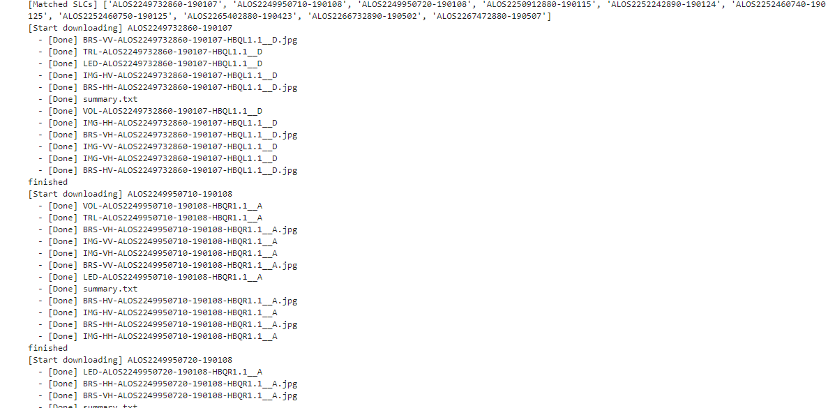
target_ids = [_['dataset_id'] for _ in target_places_json]Through doing this, a list of SAR images that meet our requirements is saved in a folder named “target_ids”, which is used as a reference to start the download. This time we will only be downloading “ALOS2249732860-190107”. When the download finishes, full-polarimetry SAR data can be found in a folder called “./data/ALOS2249732860-190107”.
Parsing Polarimetry CEOS
Depending on the state of the CEOS, the header information and payload may be combined, which means the data hasn’t been separated. The payload is very complex data which isn’t separated into imaginary and real parts. Therefore, we have to extract the payload from the CEOS data while separating the complex data. This analysis, extraction, and separation are called parsing.
First we need to make a class for parsing SAR L1.1 named “slcinfo.py”.
class SLC_L11:
    def __init__(self, _file_name):
        self.file_name = _file_name
        self.fp = 0
        self.width = 0
        self.height = 0
        self.level = 0
        self.format = ""
        self.data = []

    def get_width(self):
        self.fp.seek(248)
        self.width = int(self.fp.read(8))

    def get_height(self):
        self.fp.seek(236)
        self.height = int(self.fp.read(8))

    def get_level(self):
        self.fp.seek(276) # if l1.1, return "544"
        self.level = int(self.fp.read(4))

    def get_format(self):
        self.fp.seek(400)
        self.format = self.fp.read(28).decode()

    def get_data(self):
        self.fp.seek(720)
        prefix_byte = 544
        data = np.zeros((self.height, self.width, 2))
        width_byte_length = prefix_byte + self.width*8 # prefix + width * byte (i32bit + q32bit)
        for i in tqdm(range(self.height)):
            data_line = struct.unpack(">%s"%(int((width_byte_length)/4))+"f", self.fp.read(int(width_byte_length)))
            data_line = np.asarray(data_line).reshape(1, -1)
            data_line = data_line[:, int(prefix_byte/4):] # float_byte:
            slc = data_line[:,::2] + 1j*data_line[:,1::2]
            data[i, :, 0] = slc.real
            data[i, :, 1] = slc.imag
        # multiplex
        self.data = data[:, :, 0] + 1j*data[:, :, 1]
        print("done")

    def parse(self):
        self.fp = open(self.file_name, mode='rb')
        self.get_width()
        self.get_height()
        self.get_level()
        self.get_format()
        self.get_data()
        self.fp.close()
        self.fp = 0
This involves performing the “parse()” function to extract image sizes and complex data from within. The part that extracts the complex data will be written in the ”get_data()” function. This retrieves the complex data from each line of the image size.
This class is used in the following manner.
import os
import struct
import numpy as np
import glob
import pickle
import gc
from slcinfo import SLC_L11

# Fields
SAVE_DIRECTORY="./data/"

# Entry point
def main():
    product_list = os.listdir(SAVE_DIRECTORY)
    for product_name in product_list:
        slc_list = glob.glob(SAVE_DIRECTORY + product_name + "/IMG-*_D")
        for slc_name in slc_list:
            print(slc_name)
            slc = SLC_L11(slc_name)
            slc.parse()
            slc.crop_data(3000, 8000, 2000) # if you use cropping,
            with open(slc_name + ".pkl", "wb") as f:
                pickle.dump(slc, f)
            slc = None
            gc.collect()

if __name__=="__main__":
       main()
Performing this parses the full-polarimetry data that was downloaded before. When this process finishes, a folder with the same name as the full-polarimetry folder with a “pkl” at the end will appear containing the parsed data.

Here is a simple explanation for the source code.
To start with, the locations of the files containing CEOS data for each of the polarized waves below has been acquired.
slc_list = glob.glob(SAVE_DIRECTORY + product_name + "/IMG-*_D")After that, the CEOS data has been parsed with the following two digits.
  slc = SLC_L11(slc_name)
            slc.parse()
The CEOS data has been truncated to prevent it from taking too much room on your HDD.
slc.crop_data(3000, 8000, 2000) # if you use cropping,After truncating it, the data will be saved as follows.
       with open(slc_name + ".pkl", "wb") as f:
                pickle.dump(slc, f)
After it has been saved, it reads the following CEOS data. In order to keep your computer from running out of memory, it deletes the data that has been saved up until now.
            slc = None
            gc.collect()
After this is finished you should have access to the following data.
IMG-HH-ALOS2249732860-190107-HBQL1.1__D
IMG-HH-ALOS2249732860-190107-HBQL1.1__D.pkl
IMG-HV-ALOS2249732860-190107-HBQL1.1__D
IMG-HV-ALOS2249732860-190107-HBQL1.1__D.pkl
IMG-VV-ALOS2249732860-190107-HBQL1.1__D
IMG-VV-ALOS2249732860-190107-HBQL1.1__D.pkl
IMG-VH-ALOS2249732860-190107-HBQL1.1__D
IMG-VH-ALOS2249732860-190107-HBQL1.1__D.pkl
Acquiring the Amount of Radar Reflections With Polarimetric Decomposition
There are two main methods of performing polarimetric decomposition depending on the hypothesized surface you are working with.
They are called “coherent decomposition” and “incoherent decomposition”.
– Coherent Decomposition:
This method is used for SAR images that are hypothesized to have scattered off of an ideal surface that doesn’t produce a lot of noise. One of the major techniques is called the “Pauli decomposition”.
Due to the way radars works, however, a type of noise unique to SAR called speckle noise caused by heat noise may occur, which may interfere with the accuracy of the hypothesis. Which brings us to the second method. 。
– Incoherent Decomposition:
This method is an approach that ignores the effect of noise created by coherent decomposition.
Before we perform polarimetric decomposition, we must perform a statistical process to decrease the amount of speckle noise mentioned above. This method is considered to work well with radars that create a lot of noise thanks to its ability to clear it out.
One of the major techniques for this is the “Freeman-Duran decomposition”.
We will try both of the techniques used for getting rid of noise to see which is better.
Pauli Decomposition(Coherent Decomposition)
These can be decomposed using the following equation.
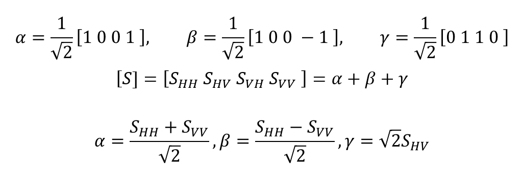
The equation is SHV=SVH with each of the components set as single reflection, double reflection, and volume scattering. It is also common to map them out in colors like using:
[α,β,ɤ]=[s,d,v]=[B,R,G]
When you use code with this programmed into it, you get the following.
%matplotlib inline
import os
import struct
import numpy as np
import glob
from tqdm import tqdm
import pickle
import cv2
import matplotlib.pyplot as plt
from slcinfo import SLC_L11
import gc

# Fields
SAVE_DIRECTORY="./data/"

def get_intensity(_slc):
    return 20*np.log10(abs(_slc)) - 83.0 - 32.0

def normalization(_x):
    return (_x-np.amin(_x))/(np.amax(_x)-np.amin(_x))

def adjust_value(_x):
    _x = np.asarray(normalization(_x)*255, dtype="uint8")
    return cv2.equalizeHist(_x)

def slc2pauli(_hh, _hv, _vv, _vh, _cross=0):
    if _cross == 0:
        _cross = (_hv + _vh) / 2
    else:
        _cross = _hv
    single = ((_hh+_vv)/np.sqrt(2)) # single, odd-bounce.
    double = ((_hh-_vv)/np.sqrt(2)) # double, even-bounce
    vol = np.sqrt(2)*_cross # vol
    return np.asarray([single, double, vol])

def grayplot(_file_name, _v):
    plt.figure()
    plt.imshow(_v, cmap = "gray")
    plt.imsave(_file_name, _v, cmap = "gray")
    print("[Save]", _file_name)

def rgbplot(_file_name, _alpha_r, _gamma_g, _beta_b):
    plttot=(np.dstack([_alpha_r, _gamma_g,_beta_b]))
    plttot=np.asarray(plttot, dtype="uint8")
    plt.figure()
    plt.imshow(plttot)
    plt.imsave(_file_name, plttot)
    print("[Save]", _file_name)
    return

# Entry point
def main():
    offset_x = 3000
    offset_y = 8000
    limit_length = 2000
    slc_hh = 0
    slc_hv = 0
    slc_vv = 0
    slc_vh = 0
    product_list = os.listdir(SAVE_DIRECTORY)
    for product_name in product_list:
        slc_list = glob.glob(SAVE_DIRECTORY + product_name + "/IMG-*.pkl")
        for slc_name in slc_list:
            with open(slc_name, "rb") as f:
                slc = pickle.load(f)
            if "IMG-HV" in slc_name:
                slc_hv = slc.data
            if "IMG-HH" in slc_name:
                slc_hh = slc.data
            if "IMG-VV" in slc_name:
                slc_vv = slc.data
            if "IMG-VH" in slc_name:
                slc_vh = slc.data
            slc_tmp = slc2intensity(slc.data)
            grayplot(slc_name + "_p.png", adjust_value(slc_tmp))
            slc = None
            gc.collect()

        ##################################
        # pauli
        ##################################
        result = slc2pauli(_hh=slc_hh, _hv=slc_hv, _vv=slc_vv, _vh=slc_vh) # alpha, beta, gmma
        [s, d, v] = get_intensity(result)
        rgbplot(SAVE_DIRECTORY + product_name + "/Pauli_decomposition.png", _alpha_r=adjust_value(d), _gamma_g=adjust_value(v), _beta_b=adjust_value(s))

if __name__=="__main__":
       main()
Performing this code gives you the following.
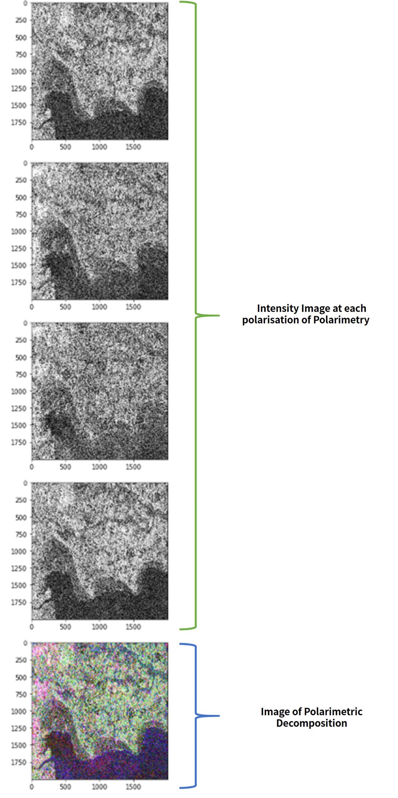
Images that have undergone polarimetric decomposition are shown after the intensity images for each of the polarities.
These are also saved into the full-polarimetry folder that contain their original images
So let us give a simple explanation for what is going on here, in terms of code.
First, we have loaded the list of full-polarimetry files from below.
slc_list = glob.glob(SAVE_DIRECTORY + product_name + "/IMG-*.pkl")Then, we have loaded each of the polarimetric decompositions for each type of polarimetry below.
 for slc_name in slc_list:
            with open(slc_name, "rb") as f:
                slc = pickle.load(f)
            if "IMG-HV" in slc_name:
                slc_hv = slc.data
            if "IMG-HH" in slc_name:
                slc_hh = slc.data
            if "IMG-VV" in slc_name:
                slc_vv = slc.data
            if "IMG-VH" in slc_name:
                slc_vh = slc.data
            slc_tmp = slc2intensity(slc.data)
            grayplot(slc_name + "_p.png", adjust_value(slc_tmp))
            slc = None
            gc.collect()
Finally, using the code below we convert the full-polarimetry data into intensity images after performing polarimetric decomposition.
    result = slc2pauli(_hh=slc_hh, _hv=slc_hv, _vv=slc_vv, _vh=slc_vh) # alpha, beta, gmma
        [s, d, v] = get_intensity(result)
        rgbplot(SAVE_DIRECTORY + product_name + "/Pauli_decomposition.png", _alpha_r=adjust_value(d), _gamma_g=adjust_value(v), _beta_b=adjust_value(s))
The specific functions that go into polarimetric decomposition can be viewed below.
def slc2pauli(_hh, _hv, _vv, _vh, _cross=0):
    if _cross == 0:
        _cross = (_hv + _vh) / 2
    else:
        _cross = _hv
    single = ((_hh+_vv)/np.sqrt(2)) # single, odd-bounce.
    double = ((_hh-_vv)/np.sqrt(2)) # double, even-bounce
    vol = np.sqrt(2)*_cross # vol
    return np.asarray([single, double, vol])
We will explain the part that uses a _cross parameter. This is a parameter that specifies the calculation method for cross-polarized waves. We have explained the relation of HV=VH for the governing equation, but in actuality the results are rarely the same due to noise. In order to keep it stable, the average is used and the waves are treated as cross-polarized waves.
To check whether or not our results are correct, we will compare them with the results we get from using a specialized software.
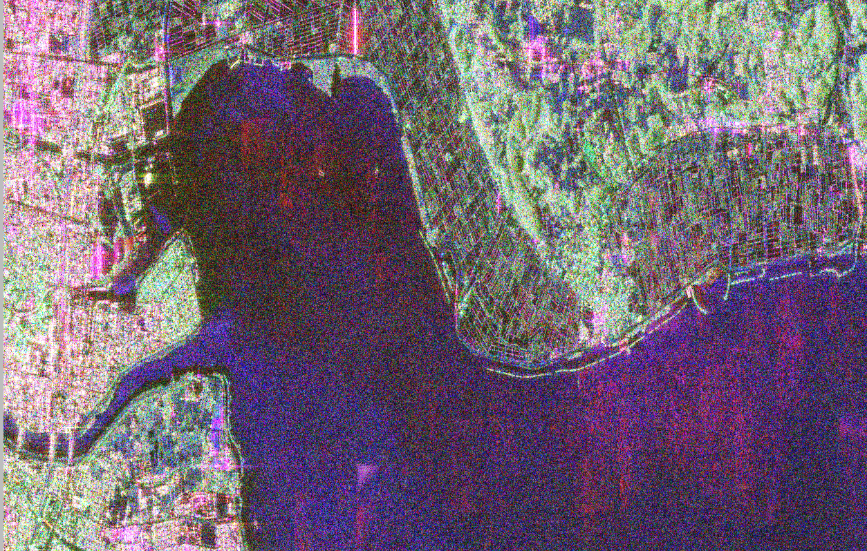
Our Code:
Specialized Software:
It seems like we have done a pretty good job, as there is very little difference between the two results.
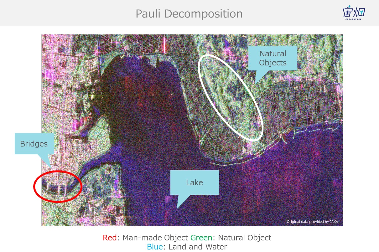
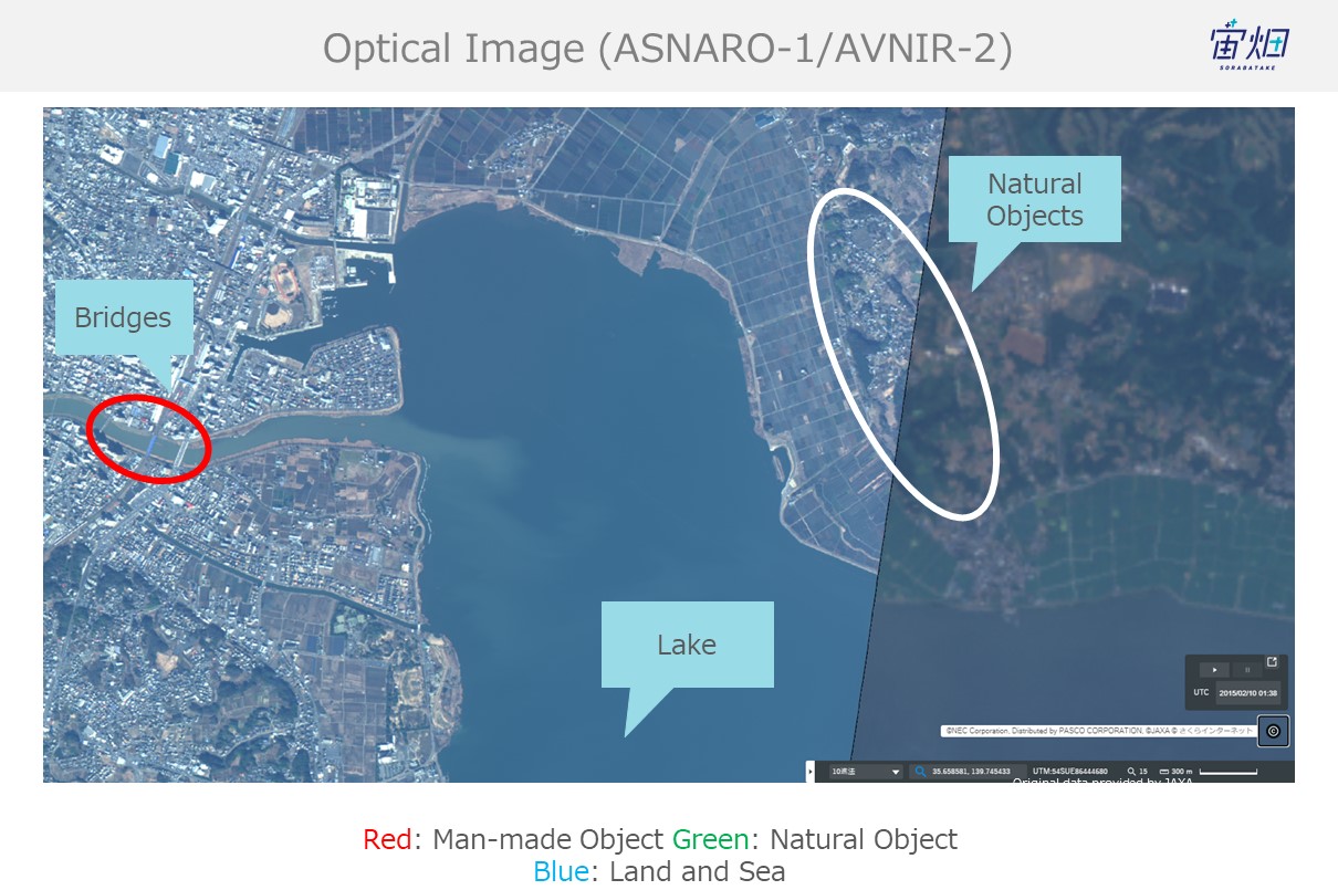
If you take a closer look at our original goal of identifying objects and classifying land coverage, you can see how man-made structures such as bridges are red (double reflection), the sea is blue (single reflection), and dirt and trees are green (volume scattering).
Freeman Duran Decomposition(Incoherent Decomposition)
Here we will perform the aforementioned statistical process used to decrease the amount of speckle noise before performing polarimetric decomposition. The polarimetric decomposition isn’t simple like the Pauli decomposition which means that there are conditional branches like the ones below. There is a lengthy explanation for why this is the case, but we will leave it out for now. For those of you who are interested, check out the original presentation.
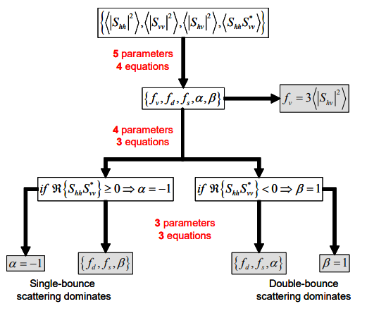
The code we used uses the following function.
*Use this in addition to the source code for the Pauli decomposition.
def slc2cov(_hh, _hv, _vv, _vh, _nb=2, _cross=0):
    [m,n] = _hh.shape
    result = np.zeros((m,n,9),dtype=np.complex64)
    if _cross == 0:
        _cross = (_hv + _vh) / 2
    else:
        _cross = _hv
    cross = cross * np.sqrt(2)
    for i in tqdm(np.arange(0, m)):
        for j in np.arange(0, n):

            i_one = np.array((0, i - _nb))
            i_two = np.array((i+_nb+1, m))

            j_one = np.array((0, j-_nb))
            j_two = np.array((j+_nb + 1, n))

            hh_tmp = np.copy(_hh[np.max(i_one):np.min(i_two),np.max(j_one):np.min(j_two)])
            vv_tmp = np.copy(_vv[np.max(i_one):np.min(i_two),np.max(j_one):np.min(j_two)])
            cross_tmp = np.copy(cross[np.max(i_one):np.min(i_two),np.max(j_one):np.min(j_two)])

            [mbis,nbis]=hh_tmp.shape

            hh_tmp = hh_tmp.reshape((mbis*nbis, 1))
            vv_tmp = vv_tmp.reshape((mbis*nbis, 1))
            cross_tmp = cross_tmp.reshape((mbis*nbis, 1))

            data = np.hstack((hh_tmp, cross_tmp, vv_tmp))

            cov = np.dot(data.T,np.conjugate(data))/(mbis*nbis)
            result[i,j,:] = cov.reshape(9,)
    return result

def cov2fdd(data):
    [m, n, p] = data.shape
    pv_array = np.zeros((m, n))
    pd_array = np.zeros((m, n))
    ps_array = np.zeros((m, n))
    for i in tqdm(np.arange(0, m)):
        for j in np.arange(0, n):
            cov=(np.copy(data[i,j,:])).reshape((3, 3))
            fv=(3*cov[1,1]/2).real
            if (cov[0,2]).real<=0:
                beta=1

                Af=(cov[0,0]-fv).real
                Bf=(cov[2,2]-fv).real
                Cf=((cov[0,2]).real-fv/3).real
                Df=(cov[0,2]).imag

                if (Af+Bf-2*Cf)!=0:
                    fd=(Df**2+(Cf-Bf)**2)/(Af+Bf-2*Cf)
                else:
                    fd=Bf

                fs=Bf-fd

                if fd!=0:
                    alpha=np.complex((Cf-Bf)/fd+1, Df/fd)
                else:
                    alpha=np.complex(1,1)

            else:
                alpha=-1

                Af=(cov[0,0]-fv).real
                Bf=(cov[2,2]-fv).real
                Cf=(cov[0,2]).real-fv/3

                if (Af+Bf+2*Cf)!=0:
                    fs=(Cf+Bf)**2/(Af+Bf+2*Cf)
                else:
                    fs=Bf

                fd=Bf-fs
                beta=(Af+Cf)/(Cf+Bf)

            pv=(8*fv/3)
            ps=(fs*(1+beta*np.conjugate(beta))).real
            pd=(fd*(1+alpha*np.conjugate(alpha))).real

            ps_array[i, j] = ps
            pd_array[i, j] = pd
            pv_array[i, j] = pv
    return np.asarray([ps_array, pd_array, pv_array])
You use it by calling the main function as follows.
        ##################################
        # freeman-duran
        ##################################
        # convert slc to cov
        cov_file_name = SAVE_DIRECTORY + product_name + "/cov.pkl"
        if not os.path.exists(cov_file_name):
            cov = slc2cov(slc_hh, slc_vv, slc_vv, slc_vh, 2)
            with open(cov_file_name, "wb") as f:
                pickle.dump(cov, f)
        with open(cov_file_name, "rb") as f:
            cov = pickle.load(f)

        # convert freeman-duran
        freeman_file_name = SAVE_DIRECTORY + product_name + "/fdd.pkl"
        if not os.path.exists(freeman_file_name):
            fdd = cov2fdd(cov)
            with open(freeman_file_name, "wb") as f:
                pickle.dump(fdd, f)
        with open(freeman_file_name, "rb") as f:
            fdd = pickle.load(f)
        [s, d, v] = get_intensity(fdd)
        rgbplot(SAVE_DIRECTORY + product_name + "/Freeman_decomposition.png", _alpha_r=adjust_value(d), _gamma_g=adjust_value(v), _beta_b=adjust_value(s))
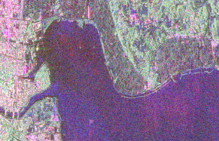
When the process finishes, it shows images that have undergone polarimetry decomposition.
Let’s compare it with our specialized software.
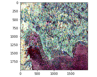
Our Code:
Specialized Software:
Since the method for converting them to RGB is different, they aren’t perfectly similar, but you can see how they both capture the same trends.
Summary
Let’s sum up today’s article and check if we were able to achieve our original goal.
Our original goal was to “perform polarimetry decomposition on SAR L1.1 data provided by PALSAR-2 to see whether or not we could accurately differentiate between natural and man-made objects.”
To see whether or not we accomplished this, we will compare the SAR images we performed polarimetry decomposition on with optical images.
Optical image:
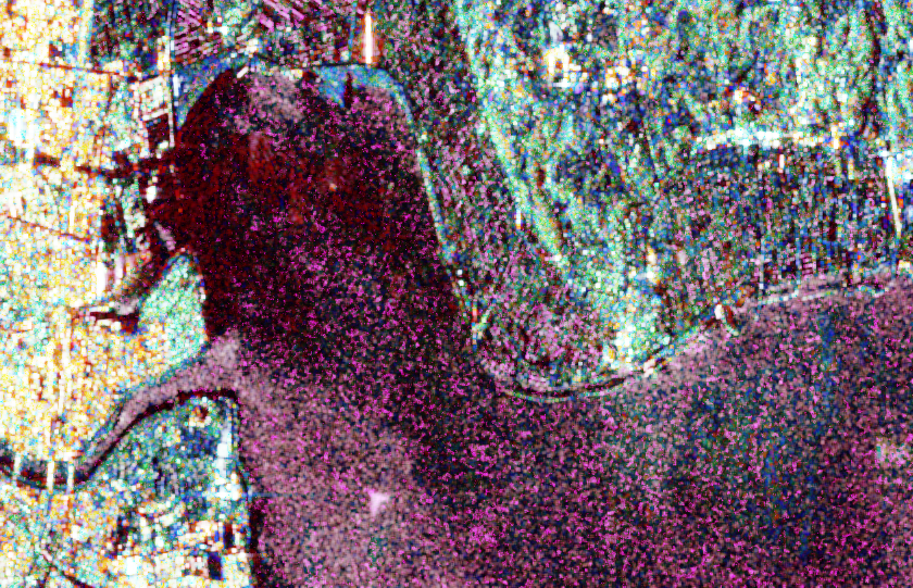
Pauli decomposition:
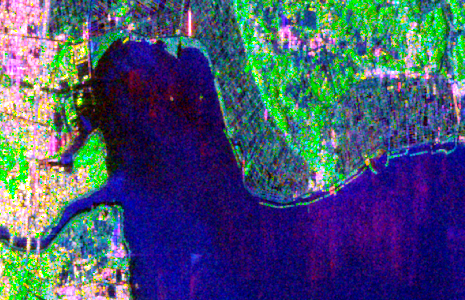
Freeman-duran decomposition:
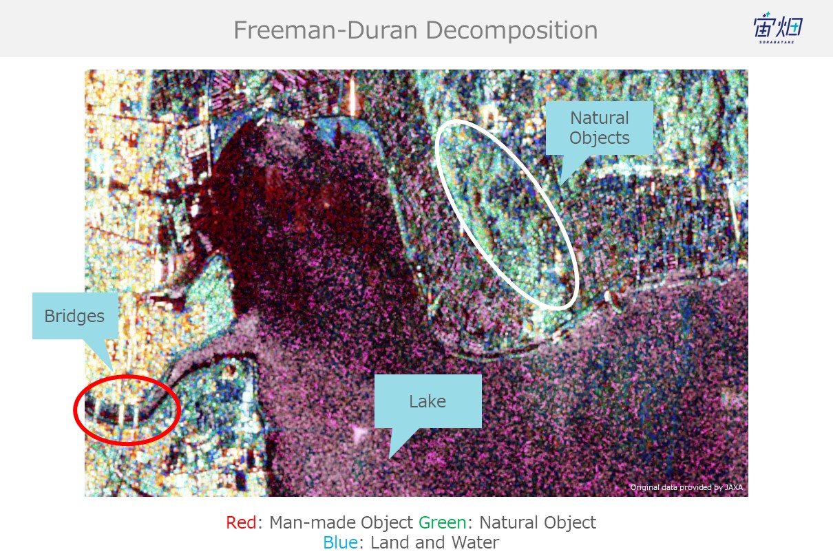
There is quite a bit of noise on the Freeman-duran version, but you can still tell the difference between natural (dirt, mountains, trees) and man-made objects.
Which means it’s safe to say that we were able to accomplish our goal.
In closing, let’s take a moment to reflect on what we went over today.
– We learned about SAR scatter processing (single reflection, double reflection, and volume reflection)
– We learned that we can acquire information on “single reflection, double reflection, and volume reflection” through performing polarimetric decomposition on full-polarimetry
– We learned that we can differentiate between simple objects using polarimetric decomposition
– We learned that we can acquire full-polarimetry CEOS (SAR L1.1) data to perform one of two different polarimetry decomposition mentions (?)
– We confirmed that our polarimetry decomposition results were accurate by comparing them with a specialized software
– We confirmed that we can classify natural and man-made objects to an extent using the polarimetry decomposition by comparing it with optical imagery
As we explained in the beginning of this article, in addition to classifying natural and man-made objects, this process can also be used to make SAR images easier to handle.
There are lots of ways to get rid of noise to make SAR images easier to handle, but the approach we take in this article allows us to add new information to the entire photo, making it a very effective way to prep.
Keep an eye out for a future article where we expand on this subject even more!