Using InSAR to Examine Mountains On Tellus [Code Included]
In this article, we will be implementing InSAR from scratch to examine subsidence. This time, we will be looking at irregular surfaces such as mountains.
The data on Tellus is collected primarily by the PALSAR-2, and SAR sensors mounted on the ALOS-2 (Daichi-2) satellite. In a previous article, we showed an example of how to use that data to create InSAR images.
Using Tellus to Determine Land Subsidence via InSAR Analysis [Code Included]
Today, we will will build up on that article by using InSAR techniques to examine mountainous parts of the earth’s surface. The algorithm we used in the previous article required us to manually remove any orbital fringe, but it isn’t possible to do this when looking at uneven surfaces. So in this article, we will be introducing a new algorithm for removing orbital fringe with estimations based on orbital fringe data.
This will allow us to extract easy-to-see terrain fringe from InSAR images of jagged terrains. Topographical fringe is, you guessed it, data (contour lines) that measures the altitude of the earth’s surface. So you can use the code in this article to create an elevation map with InSAR data! It may not be enough to use for a business endeavor or research, but hopefully it is a way for you to experience InSAR!
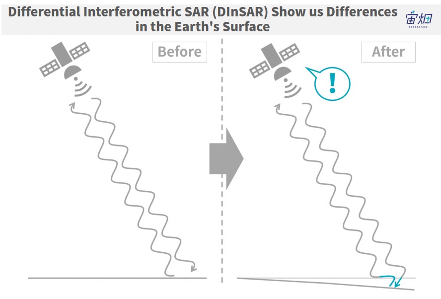
What is InSAR?
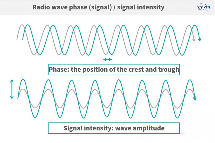
InSAR could be considered a technology that finds changes in the earth’s surface by measuring phase contrast in waves. When a satellite emits waves from a fixed position, it can detect shifts in the phases of waves reflected back at it which signify changes in the earth’s surface which may occur over a span of time.
Find out more about InSAR in this previous article where the Remote Sensing Society of Japan (RESTEC) explains it for us.
This article will focus on programming this using the Tellus development environment.
Download Interference Pairs
We explained in a previous article that there are several conditions for SAR image interference. These three conditions are that they have been captured along the same orbital trajectory (position and direction), taken in the same observational mode, and have been taken within a certain amount of time.
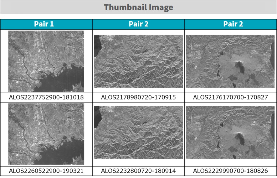
For ALOS-2, any products where their beam numbers, pass numbers, frame numbers, and observational modes all match are compatible for interference. This time, we will show you the product IDs of a few different interference pairs which we found by searching for a variety of conditions where our algorithm worked very well, so please download the following using the sample codes below.
◇Pair 1: Tokyo Bay Reclaimed Land Area
In order to prove that our algorithm for removing orbital fringe works, we’ll be using the same area from a previous article)
ALOS2237752900-181018
ALOS2260522900-190321
◇Pair 2: Kurobe Dam – Tateyama Mountain Range
ALOS2178980720-170915
ALOS2232800720-180914
◇Pair 3: Yamanakako – Mt. Fuji Areas
ALOS2176170700-170827
ALOS2229990700-180826
- Sample Code for Downloading
import os, requests

TOKEN = "ご自身のトークンを入力してください"

def publish_palsar2_l11(dataset_id):
    url = 'https://file.tellusxdp.com/api/v1/origin/publish/palsar2-l11/{}'.format(dataset_id)
    headers = {
        "Authorization": "Bearer " + TOKEN
    }
    r = requests.get(url, headers=headers)
    if not r.status_code == requests.codes.ok:
        r.raise_for_status()
    return r.json()

def download_file(url, dir, name):
    headers = {
        "Authorization": "Bearer " + TOKEN
    }
    r = requests.get(url, headers=headers, stream=True)
    if not r.status_code == requests.codes.ok:
        r.raise_for_status()
    if os.path.exists(dir) == False:
        os.makedirs(dir)
    with open(os.path.join(dir,name), "wb") as f:
        for chunk in r.iter_content(chunk_size=1024):
            f.write(chunk)

def main():
dataset_id == 'プロダクトIDをコピペしてください'
published = publish_palsar2_l11(dataset_id)
    for file in published['files']:
        file_name = file['file_name']
        file_url = file['url']
        #サムネイル画像、HH偏波の画像、サマリテキストファイル、リーダファイルのみをダウンロードします
        if "jpg" in file_name or "IMG-HH" in file_name or "summary" in file_name or "LED" in file_name:
            print(file_name)
            file = download_file(file_url, dataset_id, file_name)

if __name__=="__main__":
       main()
Once you have downloaded the images, please check to see if the thumbnails match these below, then move on to the next step.
Creating Intensity and Phase Images
We will create intensity and phase images using each of these products.
The code is almost completely identical to the one we introduced in our last article. If you try and download the entire image, it will be too large and cause a memory error, so select the ranges you want to use. The ranges are different for each pair.
Also, by creating and saving a Numpy array, then loading it in the next step, we’ve made it easier to change the code for each step of the interference analysis process. We will only mention the import modules and functions once, but they need to be used every time you run the code.
- Sample code
import os
import numpy as np
import struct
import math
from io import BytesIO
import cv2

def get_slc(fp,pl):
    fp.seek(236)
    nline = int(fp.read(8))
    fp.seek(248)
    ncell = int(fp.read(8))
    nrec = 544 + ncell*8

    nline = pl[3]-pl[2]
    fp.seek(720)
    fp.seek(int((nrec/4)*(pl[2])*4))
    data = struct.unpack(">%s"%(int((nrec*nline)/4))+"f",fp.read(int(nrec*nline)))
    data = np.array(data).reshape(-1,int(nrec/4))
    data = data[:,int(544/4):]
    data = data[:,::2] + 1j*data[:,1::2]
    data = data[:,pl[0]:pl[1]]
    sigma = 20*np.log10(abs(data)) - 83.0 - 32.0
    phase = np.angle(data)
    sigma = np.array(255*(sigma - np.amin(sigma))/(np.amax(sigma) - np.amin(sigma)),dtype="uint8")
    sigma = cv2.equalizeHist(sigma)
    return sigma, phase


def main():
    #例としてペア1を実施します。
#二つの画像に対してコメントアウトを入れ替えて2度実行してください。

    dataset_id = 'ALOS2237752900-181018'
    #dataset_id = 'ALOS2260522900-190321'

    img = open(os.path.join(dataset_id,'IMG-HH-'+dataset_id+'-UBSR1.1__D'),mode='rb')

    #範囲を指定する配列(実施するペアによって、コメントアウトを入れ替えてください)
    pl = [2500, 4500, 12000, 14000] #ペア1用
    #pl = [5000, 7500, 13000, 15500] #ペア2用
    #pl = [3750, 7450, 8500, 10500] #ペア3用

    #複素画像の取得
    sigma, phase = get_slc(img,pl)

    #強度、位相画像の出力(2つの画像に対してコメントアウトを入れ替えて二度実行)
    np.save('sigma01.npy',sigma) #numpy配列として出力
    np.save('phase01.npy',phase) #numpy配列として出力
    #np.save('sigma02.npy',sigma) #numpy配列として出力
    #np.save('phase02.npy',phase) #numpy配列として出力

    #強度画像の出力・保存
    plt.figure()
    plt.imsave('sigma.png', sigma,cmap='gray', vmin = 0, vmax = 255)
    plt.imsave('phase.png', phase,cmap='jet', vmin = 0, vmax = 255)

if __name__=="__main__":
       main()
The images we get look like this. Each pair is made up of two pictures that have nearly identical images, so we will only show the first image for each pair. For intensity images, we calibrate the reflection coefficient into a logarithm and flatten the histogram even further using OpenCV features. The phase image is then wrapped between -180 and + 180 degrees (-π to+π).
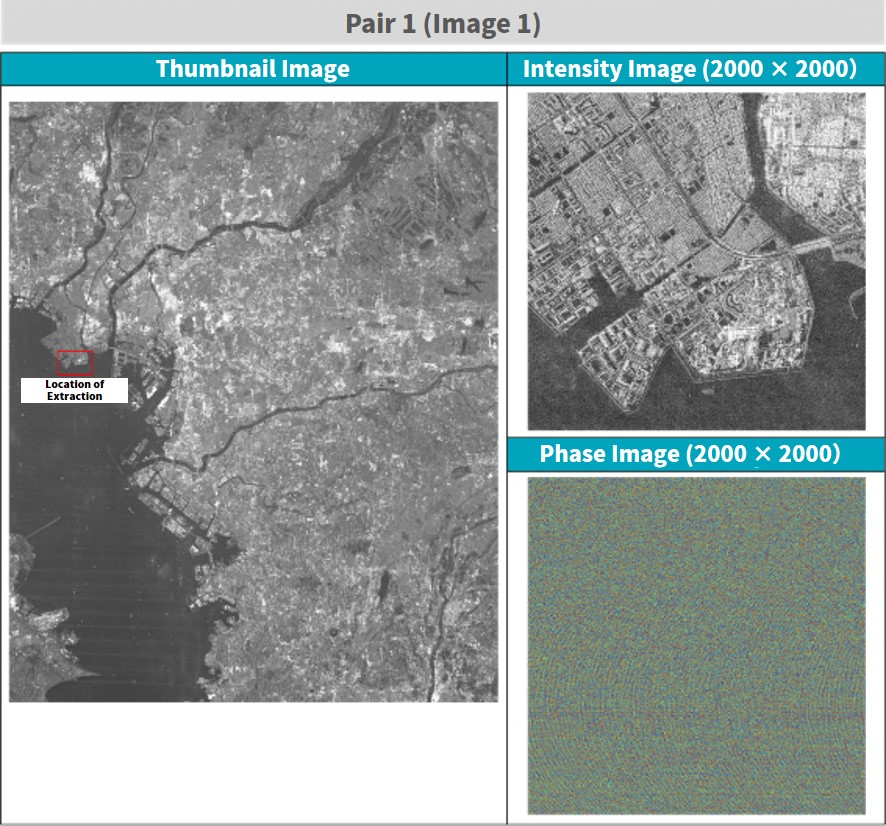
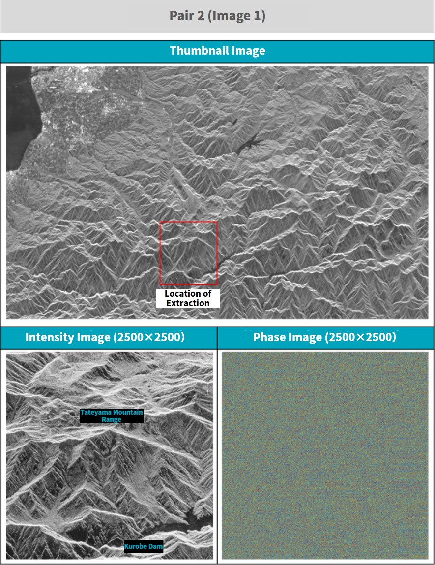
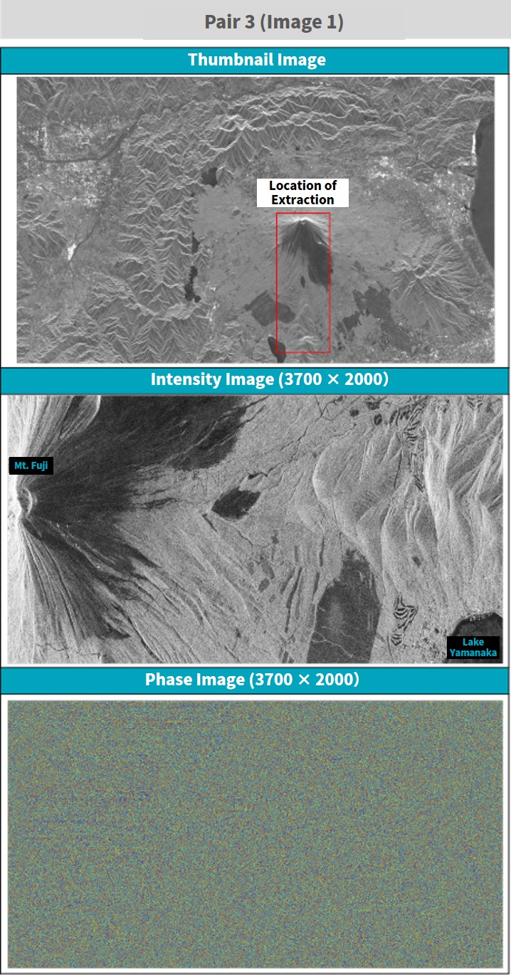
The resolution for Intensity images is 6m, which is a good resolution for being able to examine the terrain of the earth’s surface. Each image has 200 – 3700 pixels, so we recommend downloading them to view properly.
We also mentioned in our last article that phase images have no distinguishable visibility. Phase data is used to extract the difference between the two images used for interference analysis. As stated previously, however, in order to conduct an accurate interference, it is important for the location of both images to match up perfectly, which is where intensity images come into play.
Alright, so let’s use the program above to calibrate two intensity images to the same location for each pair. Once you have two phase images for each pair, we’ll move onto the next step.
Interferometric Processing
We explained what it means for two SAR images to be coherent in a previous article. To put it simply, this process uses two intensity images to find a single location, then extracts the difference in their phases. This process also uses almost the same exact code as before. Copy and paste the code below then run it.
- Sample code
#画像の位置合わせを行う関数
def coregistration(A,B,C,D):
    py = len(A)
    px = len(A[0])
    A = np.float64(A)
    B = np.float64(B)
    d, etc = cv2.phaseCorrelate(B,A)
    dx, dy = d
    if dx >= 0 and dy >= 0:
        dx = int(np.round(dx))
        dy = int(np.round(dy))
        rD = D[0:py-dy,0:px-dx]
        rC = C[dy:py,dx:px]
    elif dx = 0:
        dx = int(np.round(dx))
        dy = int(np.round(dy))
        rD = D[0:py-dy,abs(dx):px]
        rC = C[dy:py,0:px-abs(dx)]
    return rC, rD

def wraptopi(x):
    x = x - np.floor(x/(2*np.pi))*2*np.pi - np.pi
    return x

def main():
    #強度画像と位相画像の読み込み。
    phase01 = np.load('phase01.npy')
    sigma01 = np.load('sigma01.npy')
    phase02 = np.load('phase02.npy')
    sigma02 = np.load('sigma02.npy')

    coreg_phase01, coreg_phase02 = coregistration(sigma01,sigma02,phase01,phase02)
    ifgm = wraptopi(coreg_phase01 - coreg_phase03)

    np.save('ifgm.npy',ifgm01)
    plt.imsave('ifgm.jpg', ifgm, cmap = "jet")

if __name__=="__main__":
       main()
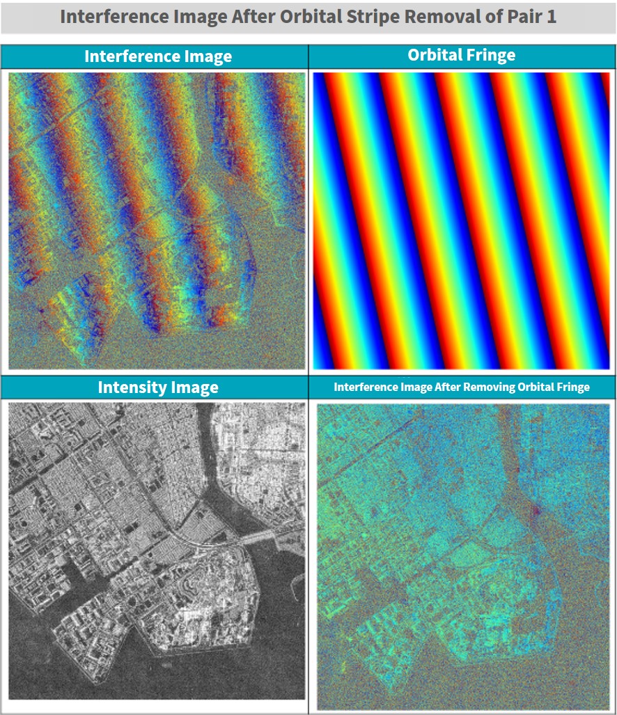
The images we get are called interferograms and can be seen below.
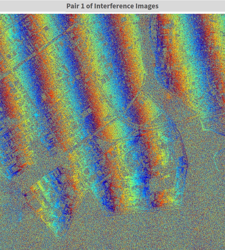
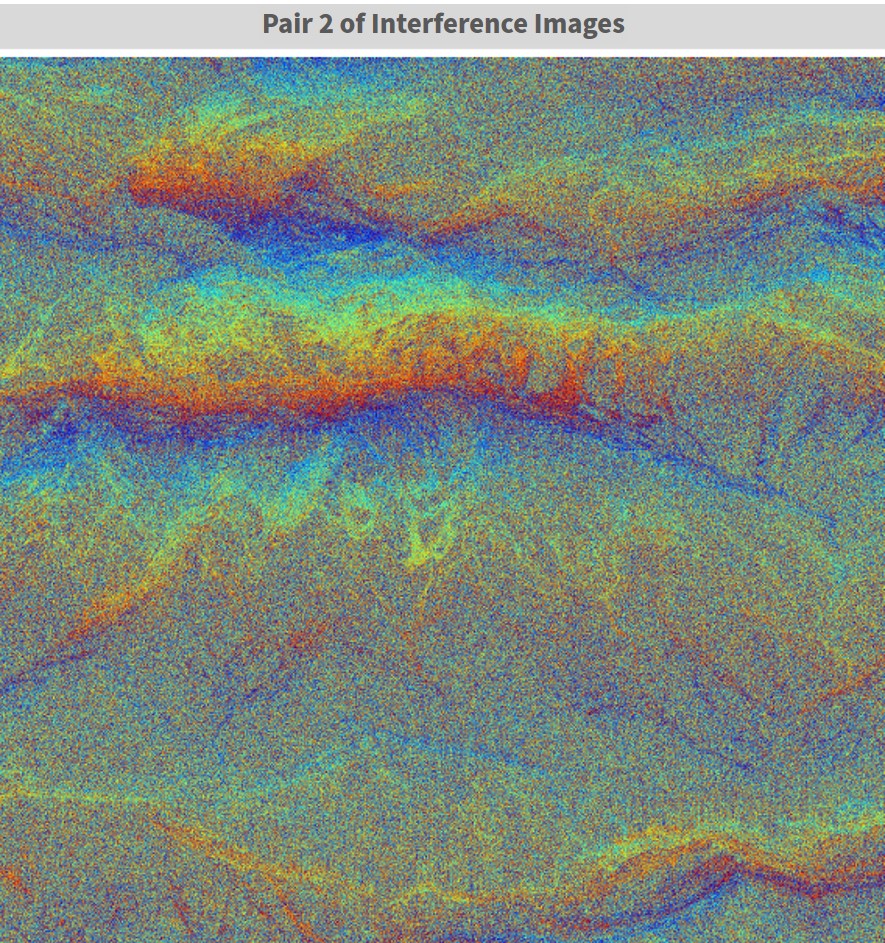
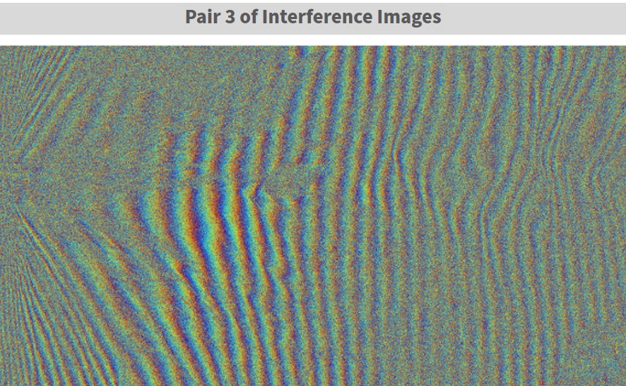
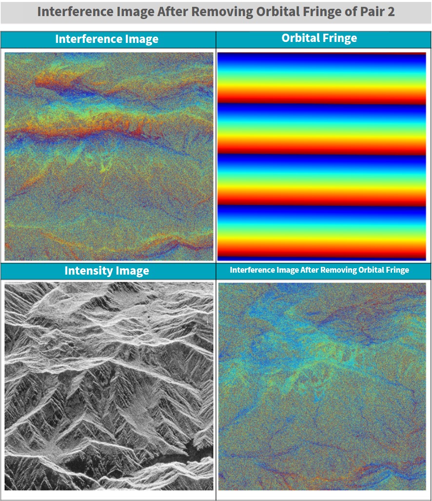
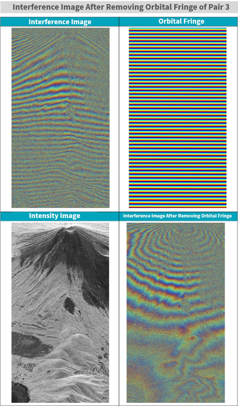
You can see here, like for pair 1 where we look at the reclaimed area of Tokyo Bay, that since it is a very flat surface, there is a uniform striped pattern left behind. This is called orbital fringe, and just like we introduced in our previous article for a uniform orbital fringe like this, it is possible to create and remove the orbital fringe by looking at the images with your own eyes. But for pairs 2 and 3, where we have more uneven, mountainous surfaces, the topographical fringe and orbital fringe mix together, making it impossible to tell just by looking at it.
That is where you can use the algorithm introduced in this article to make an estimate of the orbital fringe using the orbital data saved within the standard SAR product. Through doing this you will be able to remove the orbital fringe and get an image that shows just the topographical fringe for the area you are looking at.
The Main Theme of This Article: Using Orbital Information to Remove Orbital Fringe!
Building up on our previous article, let’s explain what orbital fringe is in a little bit more detail.
Orbital fringe occurs when the satellite’s position changes ever so slightly between observations. To be more precise, the phase part of orbital fringe is the difference between the earth’s surface and the satellite divided by the wavelength of the radar. It might be a little hard to understand by just hearing an explanation, so here is a graph to help you understand.
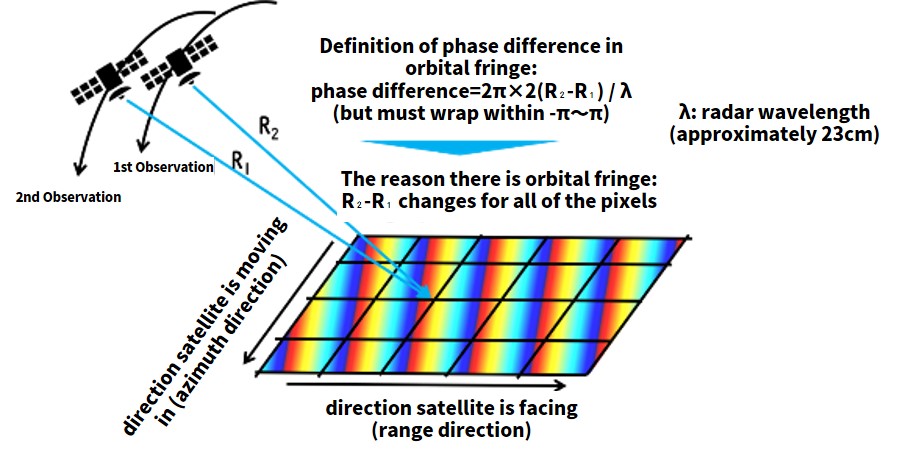
SAR images also tend to take about ten seconds to capture a single image. The satellites move a distance of about 100km during that 10 seconds, and the distance they move can’t be ignored. So in order to figure out where the satellite was when it took each part of the image, we use the time and position data recorded by the satellite to interpolate its position. The data is saved in a format called CEOS (to learn more about the CEOS format, please read this article.) We hope this image helps you understand what we are talking about.
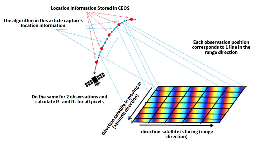
The actual algorithm used to run the CEOS format is very complex, so it’s okay if you don’t completely understand it. What’s important is that you are able to acquire accurate orbital fringe in the image as we explained, so if you’ve followed this up until now, try copy and pasting the code and running it.
- Sample code
import scipy
from scipy.interpolate import interp1d

#観測中の衛星位置を出力する関数
def get_sat_pos(led,img):
    img.seek(720+44)
    time_start = struct.unpack(">i",img.read(4))[0]/1000
    led.seek(720+500)
    lam = float(led.read(16)) #m

    led.seek(720+4096+140)
    position_num = int(led.read(4))
    led.seek(720+4096+182)
    time_interval = int(float(led.read(22)))

    led.seek(720+4096+160)
    start_time = float(led.read(22))

    led.seek(720+68)
    center_time = led.read(32)
    Hr = float(center_time[8:10])*3600
    Min = float(center_time[10:12])*60
    Sec = float(center_time[12:14])
    msec = float(center_time[14:17])*1e-3
    center_time = Hr+Min+Sec+msec;
    time_end = time_start + (center_time - time_start)*2;

    img.seek(236)
    nline = int(img.read(8))
    time_obs = np.arange(time_start, time_end, (time_end - time_start)/nline)
    time_pos = np.arange(start_time, start_time+time_interval*position_num,time_interval)
    pos_ary = [];

    led.seek(720+4096+386)
    for i in range(position_num):
        for j in range(3):
            pos = float(led.read(22))
            pos_ary.append(pos)
        led.read(66)
    pos_ary = np.array(pos_ary).reshape(-1,3)

    fx = scipy.interpolate.interp1d(time_pos,pos_ary[:,0],kind="cubic")
    fy = scipy.interpolate.interp1d(time_pos,pos_ary[:,1],kind="cubic")
    fz = scipy.interpolate.interp1d(time_pos,pos_ary[:,2],kind="cubic")
    X = fx(time_obs)
    Y = fy(time_obs)
    Z = fz(time_obs)
    XYZ = np.zeros(nline*3).reshape(-1,3)
    XYZ[:,0] = X
    XYZ[:,1] = Y
    XYZ[:,2] = Z
    return XYZ

#軌道縞を生成する関数
def get_orbit_stripe(pos1,pos2,pl,led):
    led.seek(720+500)
    lam = float(led.read(16)) # [m]
    a = []
    b = []
    c = []
    led.seek(720+4096+1620+4680+16384+9860+325000+511000+3072+728000+1024)
    for i in range(25):
        a.append(float(led.read(20)))
    for i in range(25):
        b.append(float(led.read(20)))
    for i in range(2):
        c.append(float(led.read(20)))
    npix = pl[1]-pl[0]
    nline = pl[3]-pl[2]
    orb = np.zeros((nline,npix))
    for i in range(npix):
        if i % 100 == 0:
            print(i)
        for j in range(nline):
            px = i+pl[0]-c[0]
            ln = j+pl[2]-c[1]
            ilat = (a[0]*ln**4 + a[1]*ln**3 + a[2]*ln**2 + a[3]*ln + a[4])*px**4 + (a[5]*ln**4 + a[6]*ln**3 + a[7]*ln**2 + a[8]*ln + a[9])*px**3 + (a[10]*ln**4 + a[11]*ln**3 + a[12]*ln**2 + a[13]*ln + a[14])*px**2 + (a[15]*ln**4 + a[16]*ln**3 + a[17]*ln**2 + a[18]*ln + a[19])*px + a[20]*ln**4 + a[21]*ln**3 + a[22]*ln**2 + a[23]*ln + a[24]
            ilon = (b[0]*ln**4 + b[1]*ln**3 + b[2]*ln**2 + b[3]*ln + b[4])*px**4 + (b[5]*ln**4 + b[6]*ln**3 + b[7]*ln**2 + b[8]*ln + b[9])*px**3 + (b[10]*ln**4 + b[11]*ln**3 + b[12]*ln**2 + b[13]*ln + b[14])*px**2 + (b[15]*ln**4 + b[16]*ln**3 + b[17]*ln**2 + b[18]*ln + b[19])*px + b[20]*ln**4 + b[21]*ln**3 + b[22]*ln**2 + b[23]*ln + b[24]
            ixyz = lla2ecef(ilat*np.pi/180.0,ilon*np.pi/180.0,0)
            r1 = np.linalg.norm(pos1[j+pl[2],:] - ixyz);
            r2 = np.linalg.norm(pos2[j+pl[2],:] - ixyz);
            orb[j,i] = wraptopi(2*np.pi/lam*2*(r2-r1));
    return orb

#緯度経度高度から地球のECEF座標系のXYZを出力する関数
def lla2ecef(lat,lon,alt):
    a = 6378137.0
    f = 1 / 298.257223563
    e2 = 1 - (1 - f) * (1 - f)
    v = a / math.sqrt(1 - e2 * math.sin(lat) * math.sin(lat))

    x = (v + alt) * math.cos(lat) * math.cos(lon)
    y = (v + alt) * math.cos(lat) * math.sin(lon)
    z = (v * (1 - e2) + alt) * math.sin(lat)
    return np.array([x,y,z])

def main():
    dataset_id = 'ALOS2237752900-181018' #ペア1の1枚目
    fpimg = open(os.path.join(dataset_id,'IMG-HH-'+dataset_id+'-UBSR1.1__D'),mode='rb')
    fpled = open(os.path.join(dataset_id,'LED-'+dataset_id+'-UBSR1.1__D'),mode='rb')
    pos1 = get_sat_pos(fpled,fpimg)

    dataset_id = 'ALOS2260522900-190321' #ペア1の2枚目
    fpimg = open(os.path.join(dataset_id,'IMG-HH-'+dataset_id+'-UBSR1.1__D'),mode='rb')
    fpled = open(os.path.join(dataset_id,'LED-'+dataset_id+'-UBSR1.1__D'),mode='rb')
    pos2 = get_sat_pos(fpled,fpimg)

    pl = [2500, 4500, 12000, 14000] #ペア1用
    #pl = [5000, 7500, 13000, 15500] #ペア2用
    #pl = [3750, 7450, 8500, 10500] #ペア3用

    orbit_stripe = get_orbit_stripe(pos1,pos2,pl,fpled)
    np.save('orbit_stripe.npy',orbit_stripe)

    plt.figure()
    plt.imsave('orbit_stripe.jpg', orbit_stripe, cmap = "jet")

if __name__=="__main__":
       main()
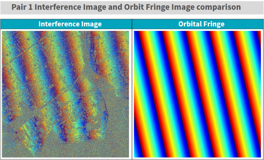
When you run the program, you should get the following orbital fringe image for pair 1. Since the earth’s surface is flat for pair 1, the fringe should be almost the same as the interference fringe. This means that you are ready to get rid of the orbital fringe.
Removing Orbital Fringe
So let’s remove the orbital fringe and see whether or not we are left with nice and neat topographical fringe. The sample code is pretty simple, you just need to subtract the prepared interferogram and orbital fringe, then wrap them into [-π~π].
def main():
    ifgm = np.load('ifgm.npy')
    orbit_stripe = np.load('orbit_stripe.npy')

  #軌道縞の画像サイズをインターフェログラムのサイズと合わせます
    orbit_stripe = orbit_stripe[0:ifgm.shape[0],0:ifgm.shape[1]]
    ifgm_sub_orb = wraptopi(ifgm - orbit_stripe) #軌道縞除去の処理

    plt.figure()
    plt.imsave('ifgm_sub_orb.jpg', ifgm_sub_orb, cmap = "jet")

if __name__=="__main__":
       main()
Let’s use pair 1 first to see how well they match up.
You can see how we were able to remove the orbital fringe quite nicely. It is also nearly identical to the image we got from our previous article, so it could be assumed that it is quite accurate as well.
Now we will put it to the real test by using it on uneven terrains, such as mountain ranges. To make our output images look more natural, we may have to shift them up or down, or to the left or right.
How to View the Interferogram After Removing Orbital Fringe
Now that we have processed the images, let’s take a moment to think about what you can learn from an interferogram that has had its orbital fringe removed. First, please think of interferograms without their orbital fringe as showing their topographical fringe. Topographical fringe could also be considered contour lines. You can use this to examine elevation of different areas using SAR data.
Let’s try it! The formula you will find in textbooks for converting a single period of topographical fringe into elevation data can be seen below. The meaning of the symbols are as the image shows.
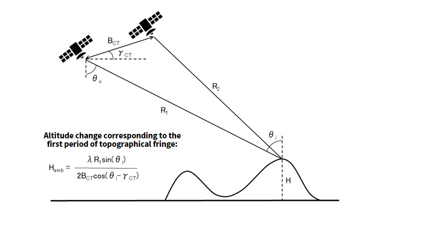
(The Basics of Synthetic Aperture Radar for Remote Sensing [The 2nd Edition] by Kazuo Ouchi, Tokyo Denki University Press, pages 230-231)
Generally speaking, values such as R1 and θi will change depending on where the pixel is within the image, so it is important to calculate it for them for different parts of the entire image, but this time we used a representative value taken from around the middle of the image.
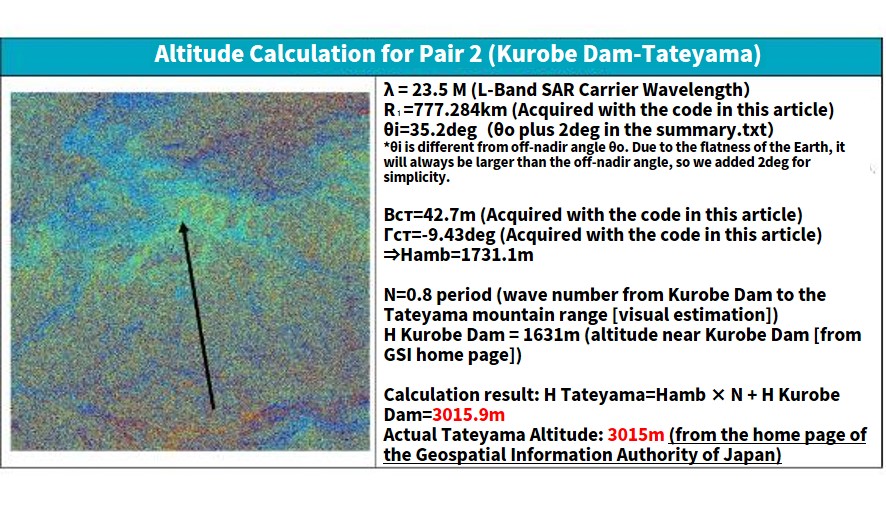
While our method to calculate these was pretty, the altitudes actually match up perfectly! For these interference images, everything was captured in one period, so the wave count (the n=0.8 part) isn’t very accurate. When we tried using the same formula for Mt. Fuji in pair number 3,
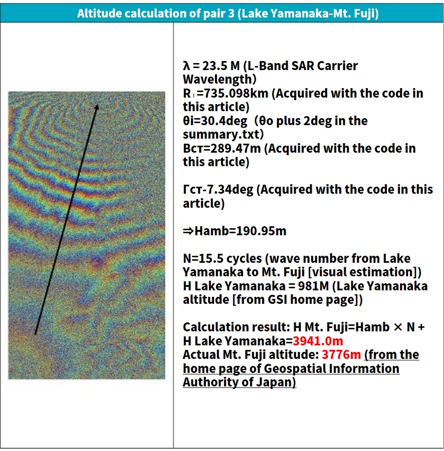
we got 3921 for its altitude. The margin of error is a bit larger than before, but it is still less than 5%, which isn’t terrible. If you were to use this formula for all parts of the image, the margin of error should stay below 5% for the altitude.
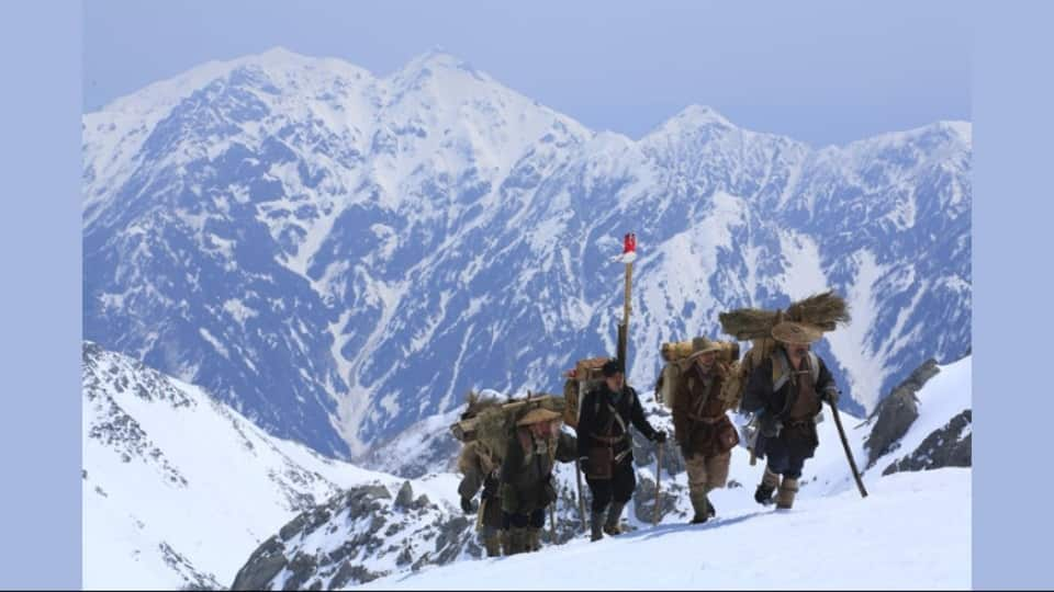
I’m personally a fan of the movie “Measuring Tsurugidake”, which shows how they used to measure the altitude of mountains, but it really puts into perspective how incredible it is we can do it from space now. Instead of climbing the mountain and measuring the difference between each spot you stop, you can measure it by looking at the surface. This is a good example of how useful space technology is.
Summary
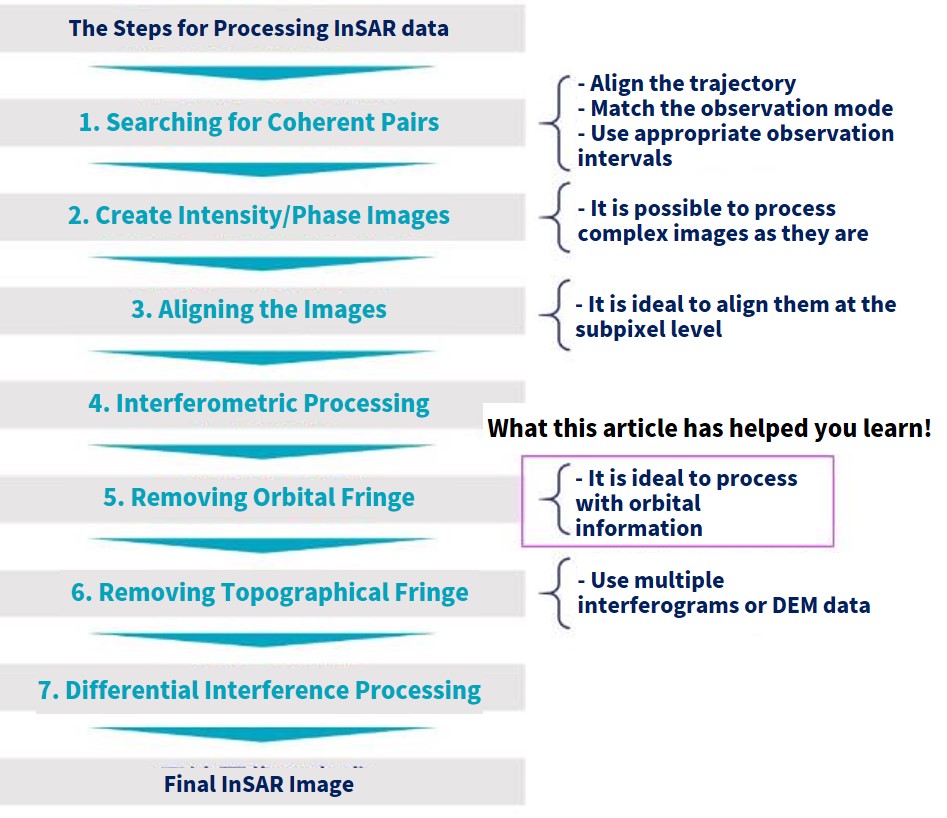
We’ve run through how to process InSAR again, which we have mentioned before in a previous article. The algorithm we introduced this time looks at the fifth step of the process, where you have to remove orbital fringe using orbital data. This will let you conduct an interference analysis on more complex terrains.
We plan on introducing more algorithms, which we hope will help you someday make your own original InSAR application. Thank you for reading!