IBM と NASA の「Largest Geospatial AI」とは? 複数衛星のデータ融合と衛星基盤モデルによる先端技術の利用とその Python実装
個別の学習なしで、様々な問題に柔軟に対応できる機械学習モデル「基盤モデル」と実装例を紹介します。
はじめに
近年のコンピュータービジョンの発展は凄まじく、またたく間に新しい手法やサービスが出てきています。衛星画像のデータも2次元画像形式のデータとして扱わせることが多く、その恩恵を受けています。
衛星データも豊富になってきた現在では、コンピュータービジョンの著しい進化に加えて、衛星独自の特性を活かした論文が出てきました。なかでも、「基盤モデル」と呼ばれる、個別の学習なしで、様々な問題に柔軟に対応できる機械学習モデルの紹介と、実装例をご紹介します。
基盤モデル
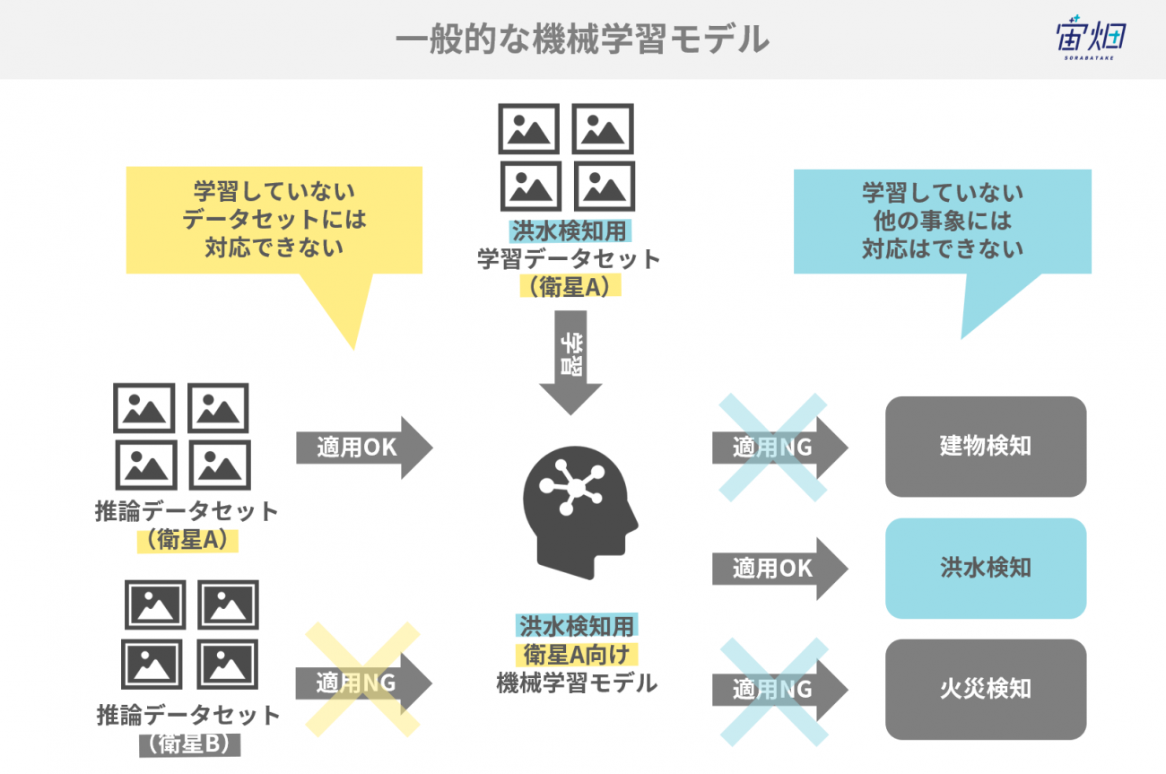
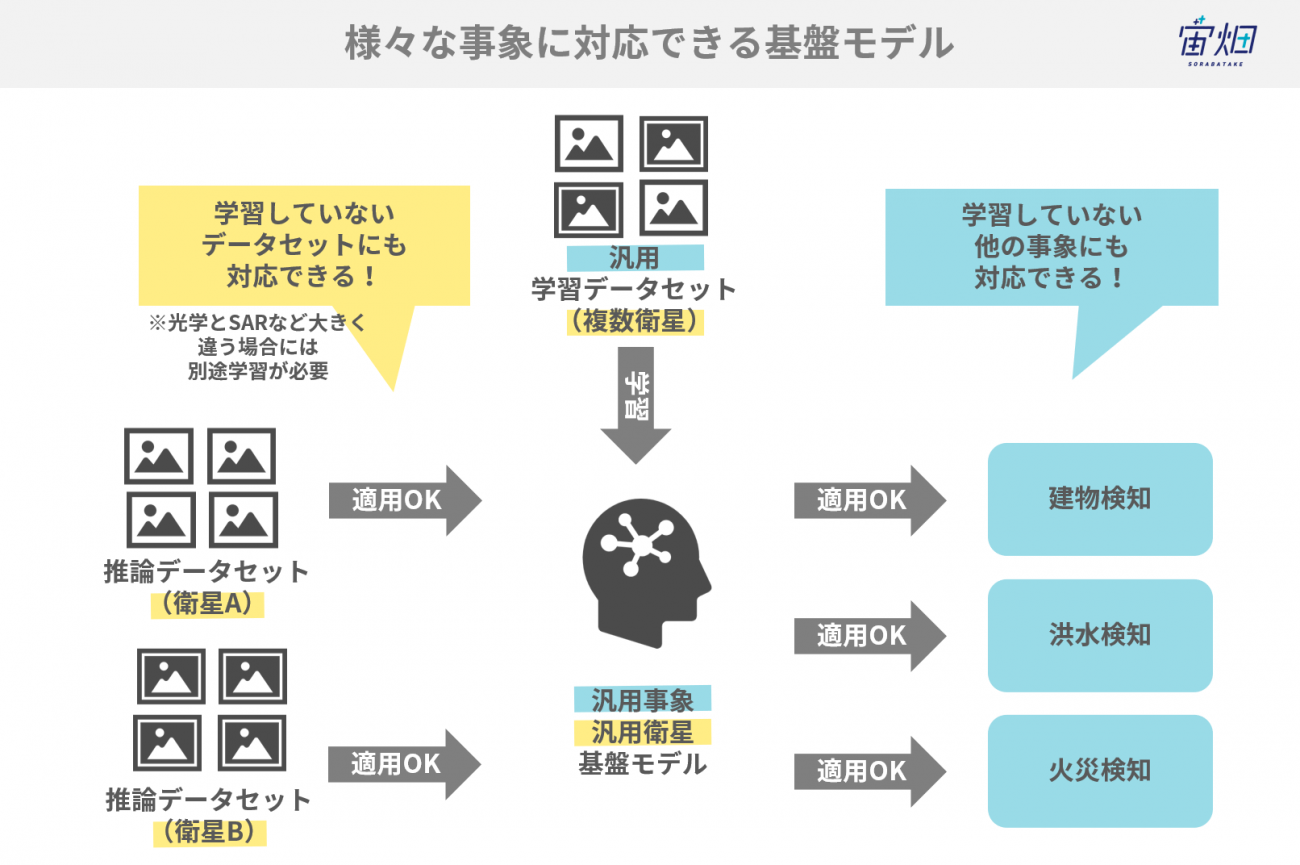
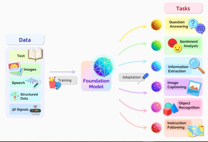
基盤モデル(Foundation Model)とは、大量データで一般的な特徴を学習したモデルのことです。人間で言う「常識」のような概念を獲得できます。特に近年、それを印象付けたブレイクスルーとしては、OpenAIのCLIPやChatGPTのGPT-4です。

事前学習モデルの利用は ImageNet で学習されたCNN(ResNet や EfficientNet など)、NLP では BERT などが古くから活かされてきました。しかし、OpenAI の事前学習モデルが一線を画すのは Zero-Shot と言われる、学習したモデルの特徴を全く調節せずに有効に使用できるということです。
これによって画像や言語分野において、人間に近いような数字の特徴量として変換できる世界になったと言えるでしょう。その世界を支えているという意味での基盤だと理解するとわかりやすいです。
地理空間基盤モデル
そして、このような基盤モデルの進化は衛星データ領域も例外ではありません。その動きの1つをご紹介します。
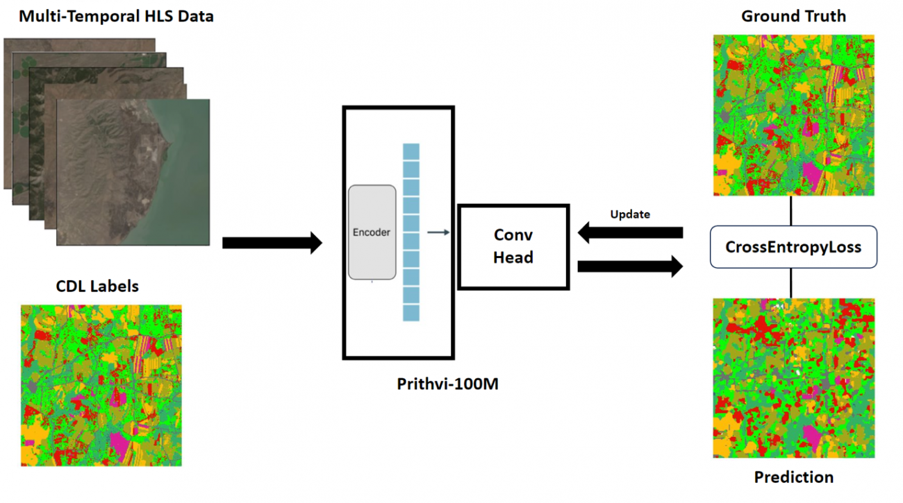
IBM と NASA が 「Largest Geospatial AI」というモデルをオープンソースにしました。これは、複数の(Landsat, Sentinel-2 の2機の)地球観測衛星のデータを融合させた地理空間版の基盤モデルです。
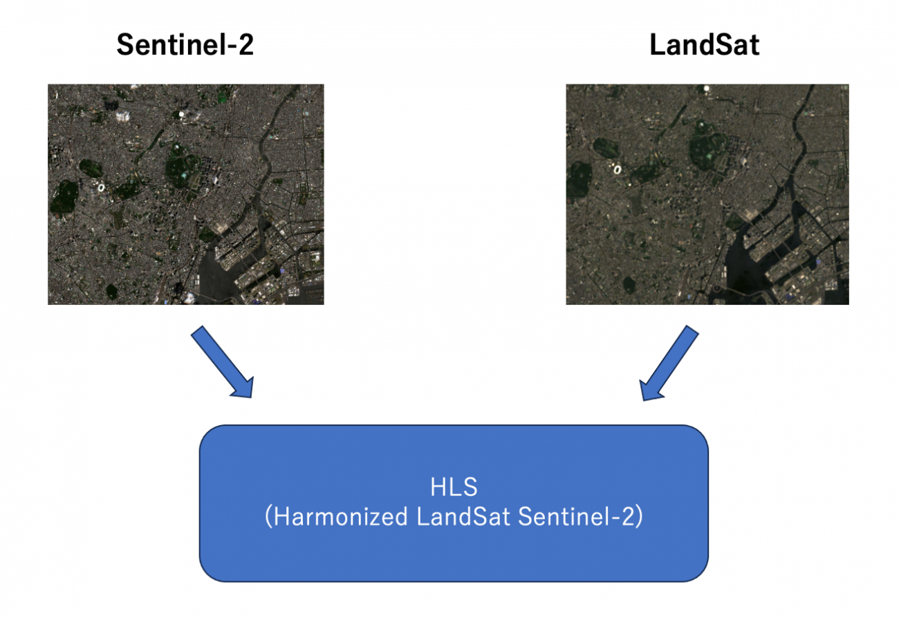
その融合させたデータをHarmonized LandSat Sentinel-2(HLS) と呼んでいます。
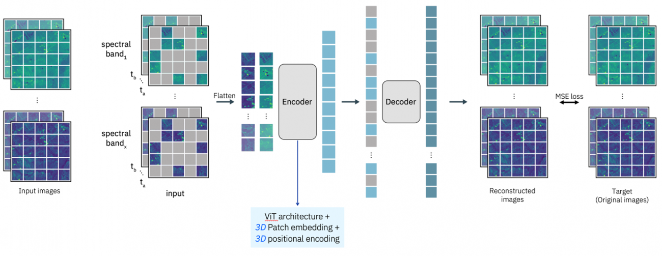
HLS を用いてTransformer ベースの画像モデルである ViTVision TransformerをMAE (Masked AutoEncoder)の構成で学習しています。
地理空間的な情報をより強調させるためか、撮像データを時系列に 3D 構造で学習できるように拡張されています。
このモデルはすでに火事検知、洪水検知、土壌被覆観測といった下流のモデルに利用されています。災害時や、農業での利用など、その他の様々な事例に使えそうですね。
利用衛星データ
今回は大規模な Sentinel-1, Sentinel-2 の画像ペアデータセット ( SEN12MS-CR DATASET, SEN12MS-CR-TS DATASET )を利用します。
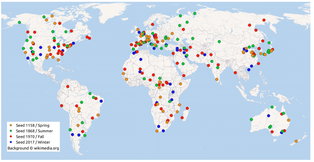
これらは世界各国の様々な時期のデータと時系列の衛星データのセットが提供されています。
データが多いので春季の画像を選択します。
PATH_ROOT = f'../sample/'


S1 = f'{PATH_ROOT}ROIs1158_spring_s1/'
S2 = f'{PATH_ROOT}ROIs1158_spring_s2/'
S2_CLOUDY = f'{PATH_ROOT}ROIs1158_spring_s2_cloudy/'


PATH_OUTPUT = f'output/'
os.makedirs(PATH_OUTPUT, exist_ok=True)
春季の一覧をみましょう。
PATHS_TIF_S1 = sorted(glob(os.path.join(S1, '*', '*.tif')))
PATHS_TIF_S2 = sorted(glob(os.path.join(S2, '*', '*.tif')))
PATHS_TIF_S2_CLOUDY = sorted(glob(os.path.join(S2_CLOUDY, '*', '*.tif')))


assert len(PATHS_TIF_S1) == len(PATHS_TIF_S2) == len(PATHS_TIF_S2_CLOUDY)


df = pd.DataFrame({
    's1': PATHS_TIF_S1,
    's2': PATHS_TIF_S2,
    's2_cloudy': PATHS_TIF_S2_CLOUDY,
})
df.head()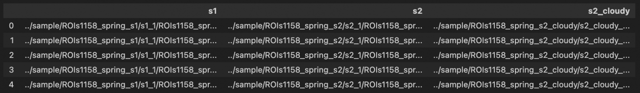
このデータをモデルのインプットにするために可視化してみます。
img_s1 = tifffile.imread(df['s1'].iloc[IDX])
print(img_s1.shape)


plt.figure(figsize=(6, 14))
for i, pol in enumerate(['VV', 'VH']):
    plt.subplot(1, 2, i+1)
    plt.title(f'Index: {IDX} Sentinel-1 {pol}', fontsize=10, fontweight='bold')
    plt.imshow(img_s1[:,:,i], cmap='gray')
plt.savefig(f'{PATH_OUTPUT}s1_{IDX}.png', bbox_inches='tight', dpi=150)
plt.show();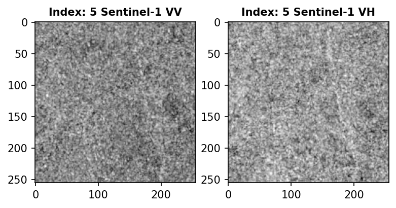
img_s2 = tifffile.imread(df['s2'].iloc[IDX])
print(img_s2.shape)


plt.figure(figsize=(24, 12), dpi=100)
for i, band in enumerate([f'Band {str(b).zfill(2)}' for b in range(1, 14)]):


    plt.subplot(3, 5, i+1)


    plt.title(f'Index: {IDX} Sentinel-2 {band}', fontsize=14, fontweight='bold')
    plt.axis('off')
    plt.imshow(img_s2[:,:,i])
plt.tight_layout()
plt.savefig(f'{PATH_OUTPUT}s2_{IDX}.png', bbox_inches='tight', dpi=150)
plt.show();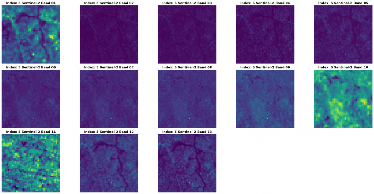
可視光波長も可視化します。
def norm_img(img):
    img = img.astype('float32')
    img = (img - img.min()) / (img.max() - img.min())
    return img


img_true = []


img_true.append(norm_img(img_s2[:,:,3]))
img_true.append(norm_img(img_s2[:,:,2]))
img_true.append(norm_img(img_s2[:,:,1]))


img_true = np.stack(img_true, axis=2)


plt.figure(figsize=(8, 8))
plt.title('Sentinel-2 True Color Image')
plt.imshow(img_true)
plt.savefig(f'{PATH_OUTPUT}true_color.png')
plt.show();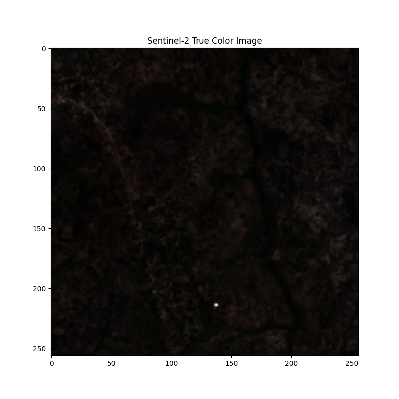
エリアを選択して可視化します。
df_area = df[df['area'] == f's1_{AREA}'][:6]


plt.figure(figsize=(20, 10))
for i in range(NUM_SAMPLE):
    PATH = df_area.iloc[i]['s2']
    img = tifffile.imread(PATH)[:,:,4]
    plt.subplot(1, 6, i+1)
    plt.imshow(img)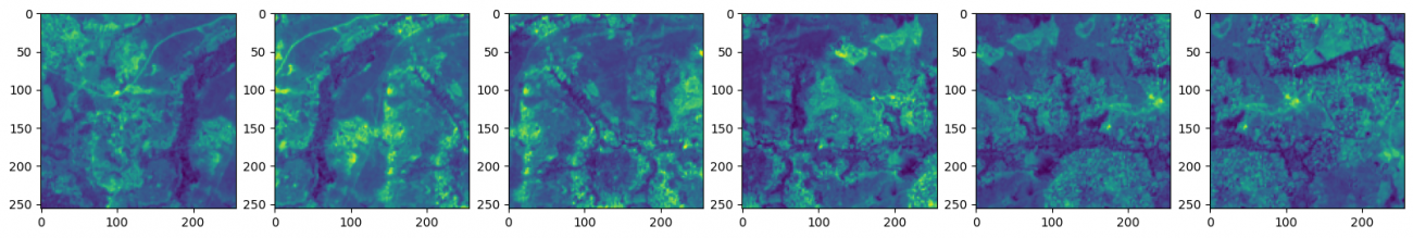
他にどんな画像があるのかを確認するために、異なるパッチを可視化してみます。
df_area = df[df['patch'] == PATCH][:6]


plt.figure(figsize=(20, 10))
for i in range(NUM_SAMPLE):
    PATH = df_area.iloc[i]['s2']
    img = tifffile.imread(PATH)[:,:,4]
    plt.subplot(1, 6, i+1)
    plt.imshow(img)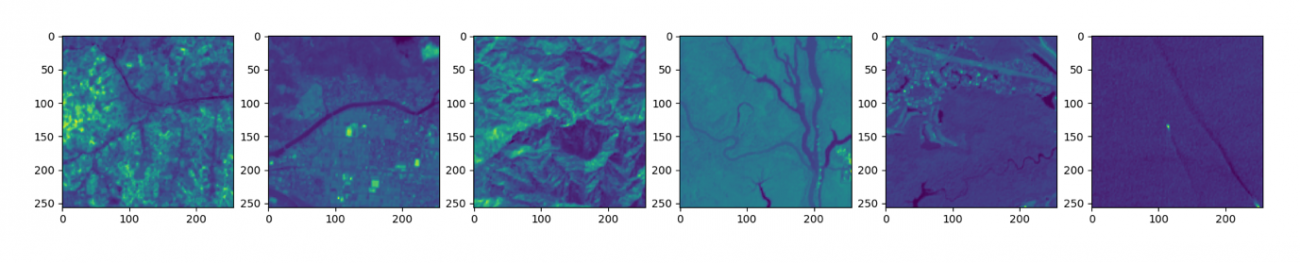
加えて、雲の領域も提供されています。
img_c = tifffile.imread(df['s2_cloudy'].iloc[IDX])
print(img_c.shape)


plt.figure(figsize=(24, 12), dpi=100)
for i, band in enumerate([f'Band {str(b).zfill(2)}' for b in range(1, 14)]):


    plt.subplot(3, 5, i+1)


    plt.title(f'Index: {IDX} Sentinel-2 {band} Cloudy', fontsize=14, fontweight='bold')
    plt.axis('off')
    plt.imshow(img_c[:,:,i])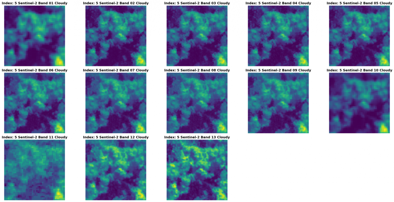
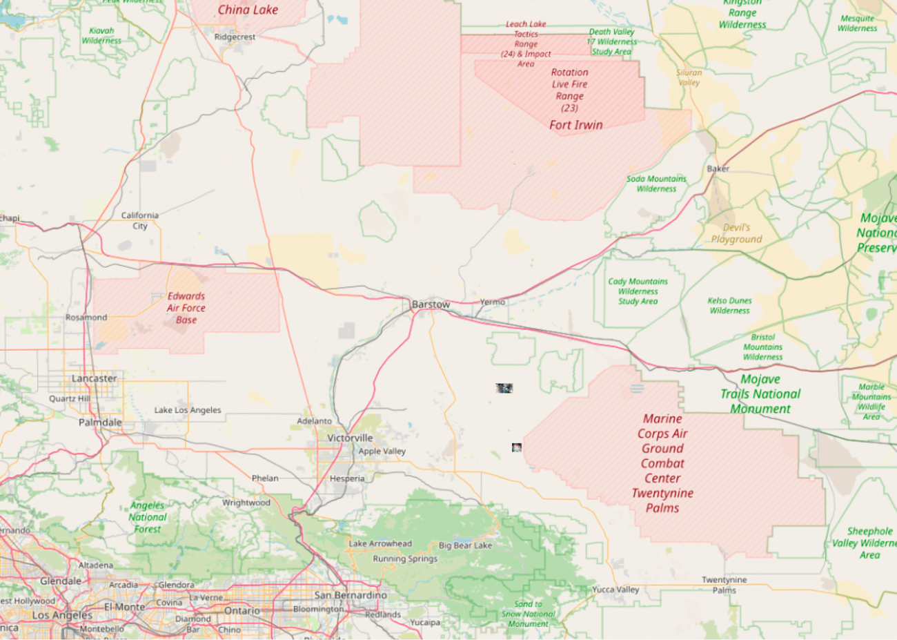
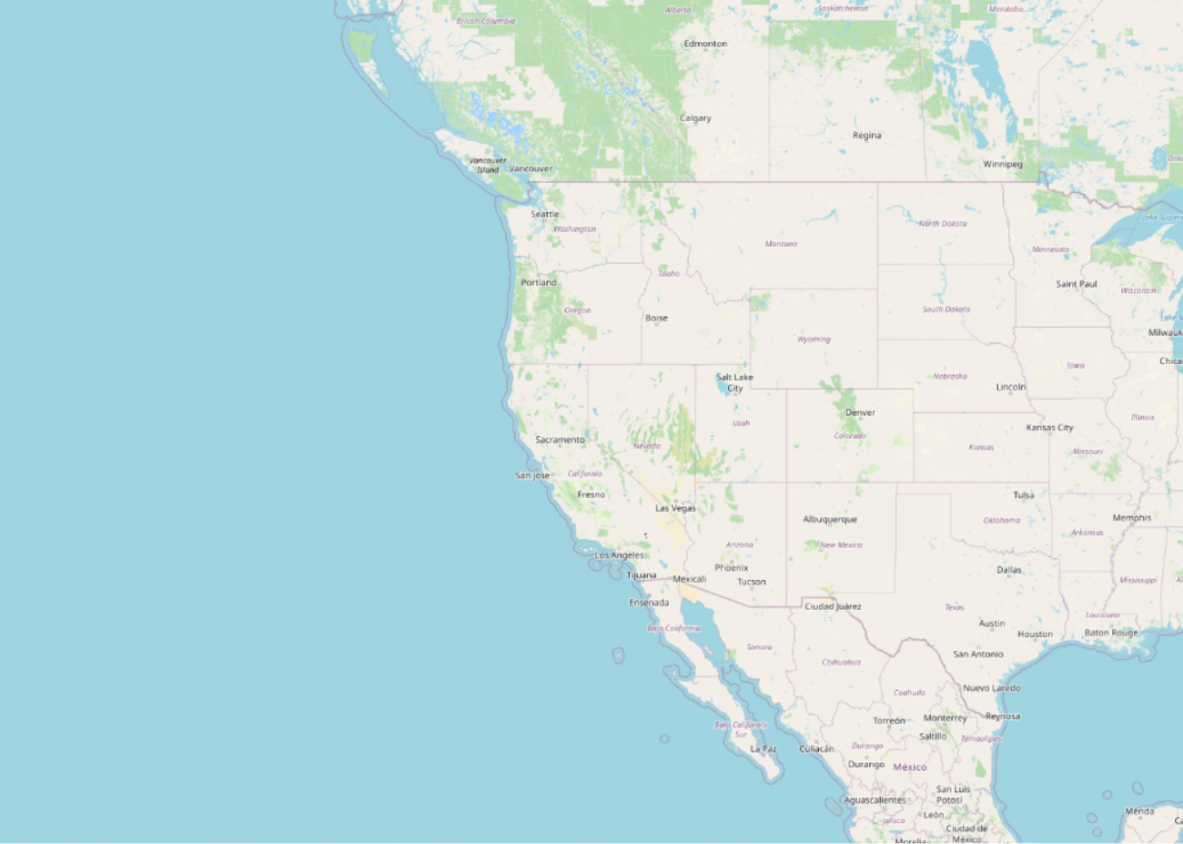
衛星データの位置情報はアメリカのロサンゼルス周辺です。
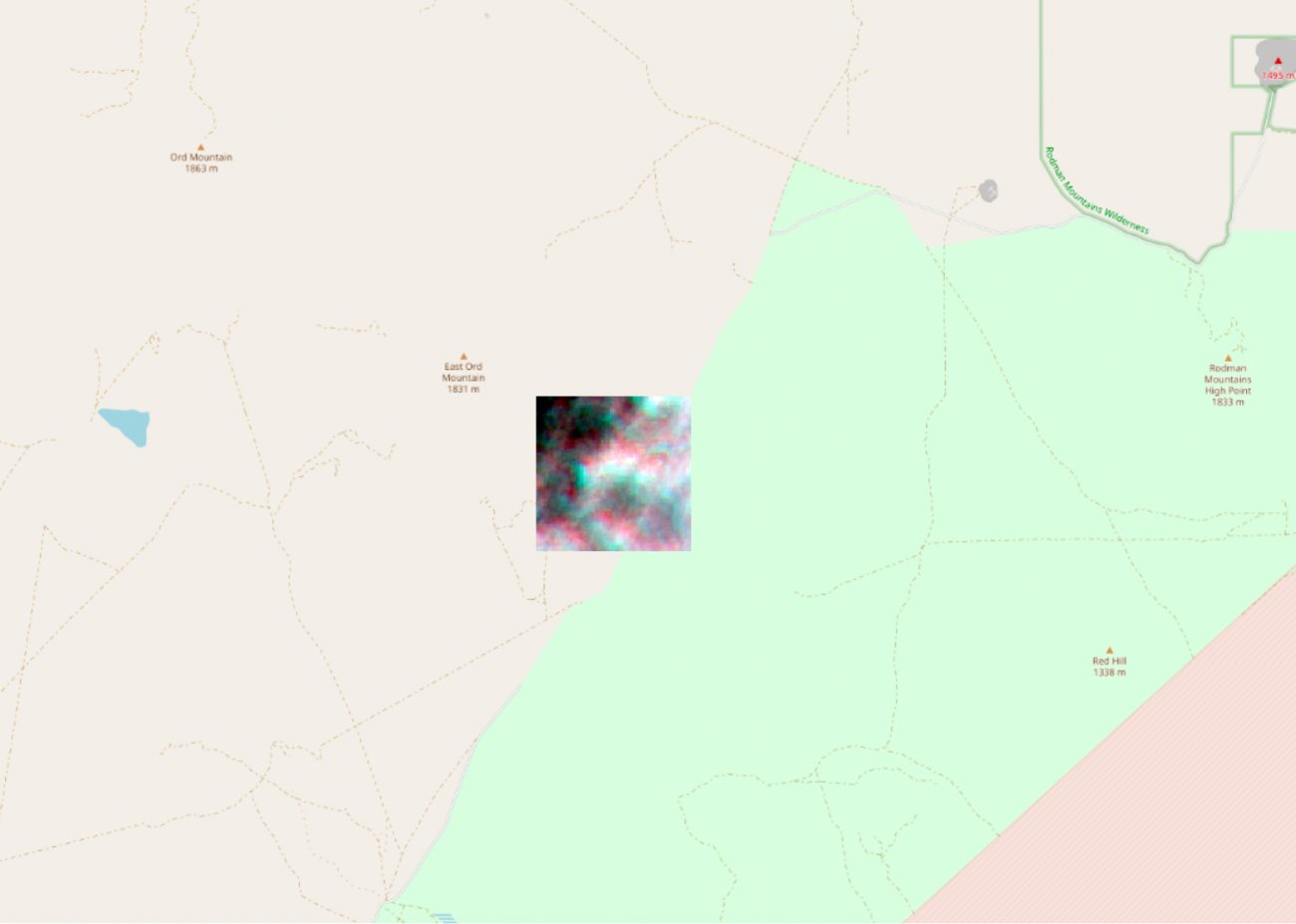
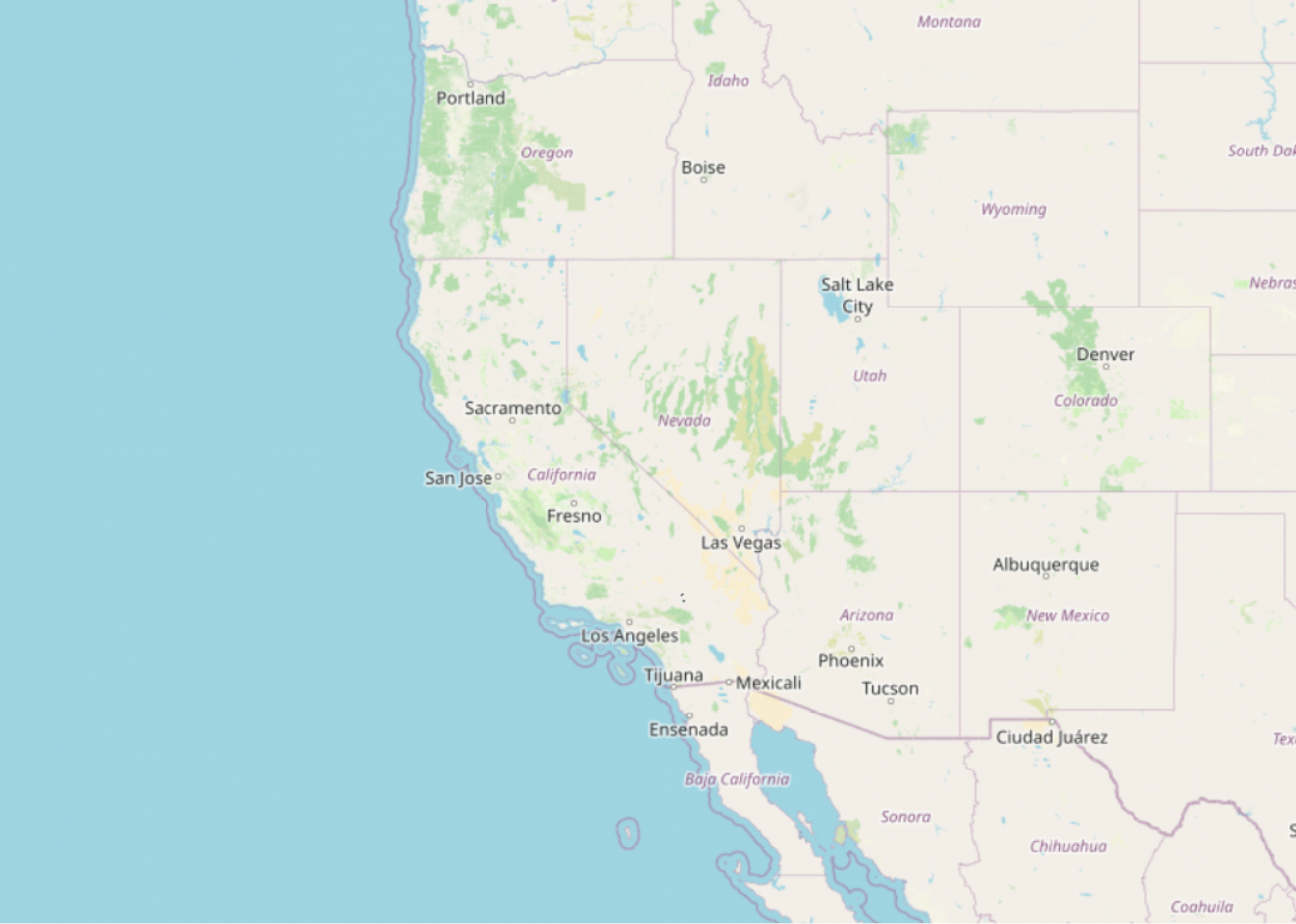
広角で見てみます。
基盤モデルの実装
では、基盤モデルから実装を確認していきます。
まずは、公開されている基盤モデルの重みを取得します。
wget https://huggingface.co/ibm-nasa-geospatial/Prithvi-100M/resolve/main/Prithvi_100M.pt -P ./pretrain/次にモデルの解像度に揃えます。
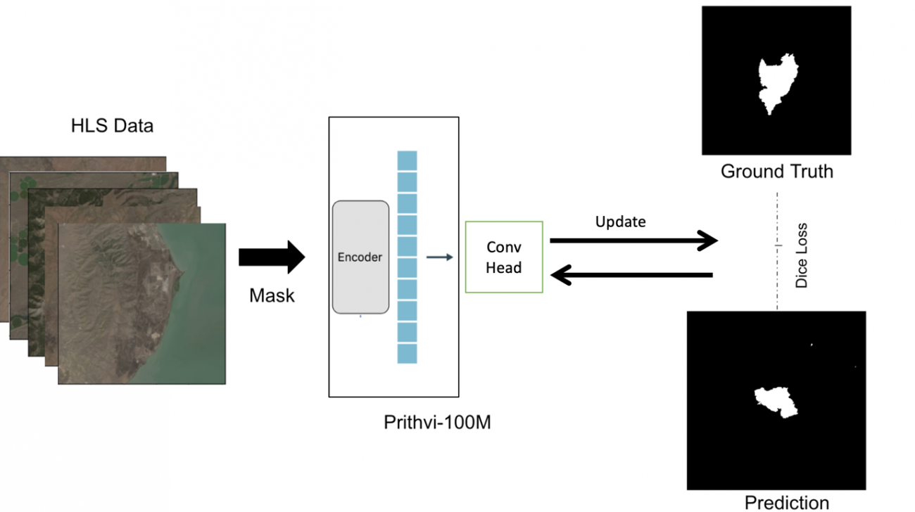
import tifffile
import cv2
import numpy as np


img = tifffile.imread('../sample/ROIs1158_spring_s2/s2_1/ROIs1158_spring_s2_1_p30.tif')
print(img.shape, img.dtype)


# 13 --> [B02, B03, B04, B05, B06, B07]
img = cv2.resize(img, (224, 224), interpolation=cv2.INTER_CUBIC)
img_band = np.stack([
    img[:, :, 1], img[:, :, 2], img[:, :, 3], # RGB
    img[:, :, 4], img[:, :, 5], img[:, :, 6],
    ],
    axis=0)


img_ts = np.stack([img_band]*3, axis=0)
print(img_ts.shape, img_ts.dtype)


# save as tif
tifffile.imwrite('../sample/ROIs1158_spring_s2/s2_1/ROIs1158_spring_s2_1_p30_resize.tif', img_ts)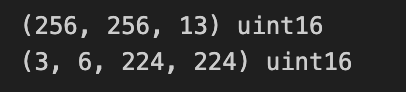
推論スクリプトを実行します。
!python 004_inference.py --data_files ../sample/ROIs1158_spring_s2/s2_1/ROIs1158_spring_s2_1_p30_resize.tif ../sample/ROIs1158_spring_s2/s2_1/ROIs1158_spring_s2_1_p30_resize.tif ../sample/ROIs1158_spring_s2/s2_1/ROIs1158_spring_s2_1_p30_resize.tif \
    --yaml_file_path ./pretrain/Prithvi_100M_config.yaml --checkpoint ./pretrain/Prithvi_100M.pt \
    --output_dir output/004/ --mask_ratio 0.5
結果を可視化してみます。
import matplotlib.pyplot as plt
pred_t0 = tifffile.imread('output/004/predicted_t0.tiff')
print(pred_t0.shape)

# plot image
plt.figure(figsize=(8, 6))
plt.subplot(1, 2, 1)
plt.title('Re Construction')
plt.imshow(pred_t0, cmap='gray')

plt.subplot(1, 2, 2)
plt.title('Ground Truth')
plt.imshow(img_ts[-1][0], cmap='gray')

# off grid
plt.tight_layout()
plt.grid(False)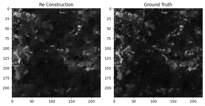
MAE の学習通りの再構成ができていることが確認できます。
Hugging Face で Web 上で試したい時は以下でデモも用意されています。
https://huggingface.co/spaces/ibm-nasa-geospatial/Prithvi-100M-demo
基盤モデルの利用
上述で紹介した基盤モデルには、火災検知、洪水検知、土壌被覆予測といった利用モデルがすでに存在します。
せっかくなのでその利用モデルもそれぞれ使用してみましょう。モデルは mmsegmentation で実装されています。環境構築でこけやすいので Notebook や公式を参考にしてください。
最初は洪水モデルです。
洪水モデルの重みを取得します。
!wget https://huggingface.co/ibm-nasa-geospatial/Prithvi-100M-sen1floods11/resolve/main/sen1floods11_Prithvi_100M.pth -P ./pretrain/洪水予測のための画像を用意します。
import tifffile
import cv2
import numpy as np

img = tifffile.imread('../../sample/ROIs1158_spring_s2/s2_1/ROIs1158_spring_s2_1_p30.tif')
print(img.shape, img.dtype)

# 13 --> 6
img = cv2.resize(img, (224, 224), interpolation=cv2.INTER_CUBIC)
img_band = np.stack([
    img[:, :, 1], img[:, :, 2], img[:, :, 3], # RGB
    img[:, :, 6], img[:, :, 11], img[:, :, 12],
    ],
    axis=0)

print(img_band.shape, img_band.dtype)

# save as tif
tifffile.imwrite('input/flood/ROIs1158_spring_s2_1_p30_flood.tif', img_band)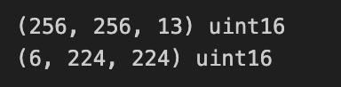
configs/sen1floods11_config.pyのファイルの以下を編集します。
- channel_last=True
+ channel_last=False
モデルに洪水の確率を推論させます。
-ckpt ../pretrain/sen1floods11_Prithvi_100M.pth \
-input input/flood/ \
-output output/flood/ -input_type tif -bands "[0,1,2,3,4,5]"
予測結果を可視化します。
PATH_OUT = f'output/flood/ROIs1158_spring_s2_1_p30_flood_pred.tif'

import matplotlib.pyplot as plt
pred_t0 = tifffile.imread(PATH_OUT)
print(pred_t0.shape)

# plot image
plt.figure(figsize=(16, 8))
plt.subplot(1, 2, 1)
plt.title('Flood')
plt.imshow(pred_t0, cmap='Blues', vmin=0, vmax=1)
plt.colorbar(shrink=0.5)

plt.subplot(1, 2, 2)
plt.title('Input')
plt.imshow(img_band[1], cmap='gray')

# off grid
plt.tight_layout()
plt.grid(False)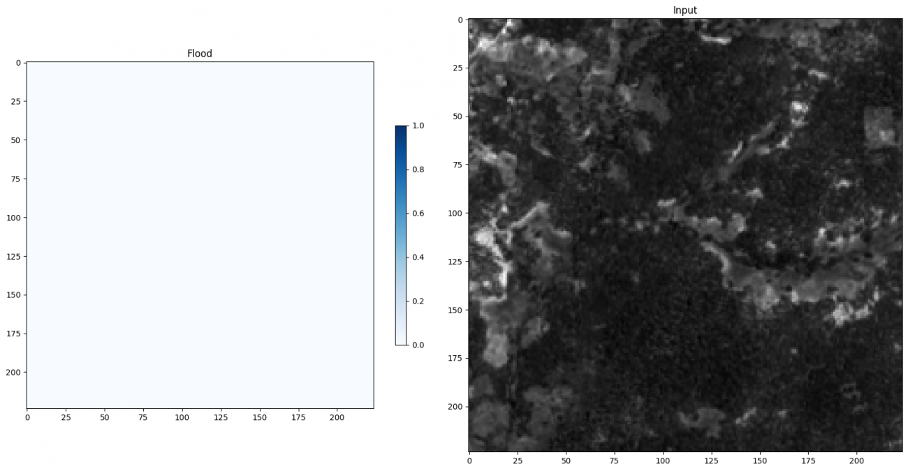
洪水が発生していないので確率が 0 (真っ白)になっています。
次に火事検知モデルです。
火事検知モデルの重みを取得します。
!wget https://huggingface.co/ibm-nasa-geospatial/Prithvi-100M-burn-scar/resolve/main/burn_scars_Prithvi_100M.pth -P ./pretrain/同様に前処理をします。
import tifffile
import cv2
import numpy as np

img = tifffile.imread('../../sample/ROIs1158_spring_s2/s2_1/ROIs1158_spring_s2_1_p30.tif')
print(img.shape, img.dtype)

# 13 --> 6
img = cv2.resize(img, (256, 256), interpolation=cv2.INTER_CUBIC)
img_band = np.stack([
    img[:, :, 1], img[:, :, 2], img[:, :, 3], # RGB
    img[:, :, 8], img[:, :, 11], img[:, :, 12],
    ],
    axis=0)

print(img_band.shape, img_band.dtype)
# img_ts = np.stack([img_band]*3, axis=0)
# print(img_ts.shape, img_ts.dtype)

# save as tif
tifffile.imwrite('input/burn/ROIs1158_spring_s2_1_p30_burn.tif', img_band)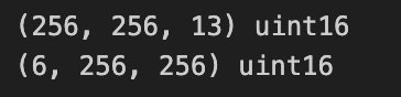
同じく設定を変更します。
configs/burn_scars.pyのファイルの以下を編集します。
- channel_last=True
+ channel_last=False
火事検知モデルを推論します。
!python model_inference.py -config configs/burn_scars.py \
    -ckpt ../pretrain/burn_scars_Prithvi_100M.pth \
    -input input/burn/ \
    -output output/burn/ -input_type tif -bands "[0,1,2,3,4,5]"
火事予測の確率も可視化します。
PATH_OUT = f'output/burn/ROIs1158_spring_s2_1_p30_burn_pred.tif'

import matplotlib.pyplot as plt
pred_t0 = tifffile.imread(PATH_OUT)
print(pred_t0.shape)

# plot image
plt.figure(figsize=(16, 8))
plt.subplot(1, 2, 1)
plt.title('Burn')
plt.imshow(pred_t0, cmap='Reds', vmin=0, vmax=1)
plt.colorbar(shrink=0.5)

plt.subplot(1, 2, 2)
plt.title('Input')
plt.imshow(img_band[2], cmap='gray')

# off grid
plt.tight_layout()
plt.grid(False)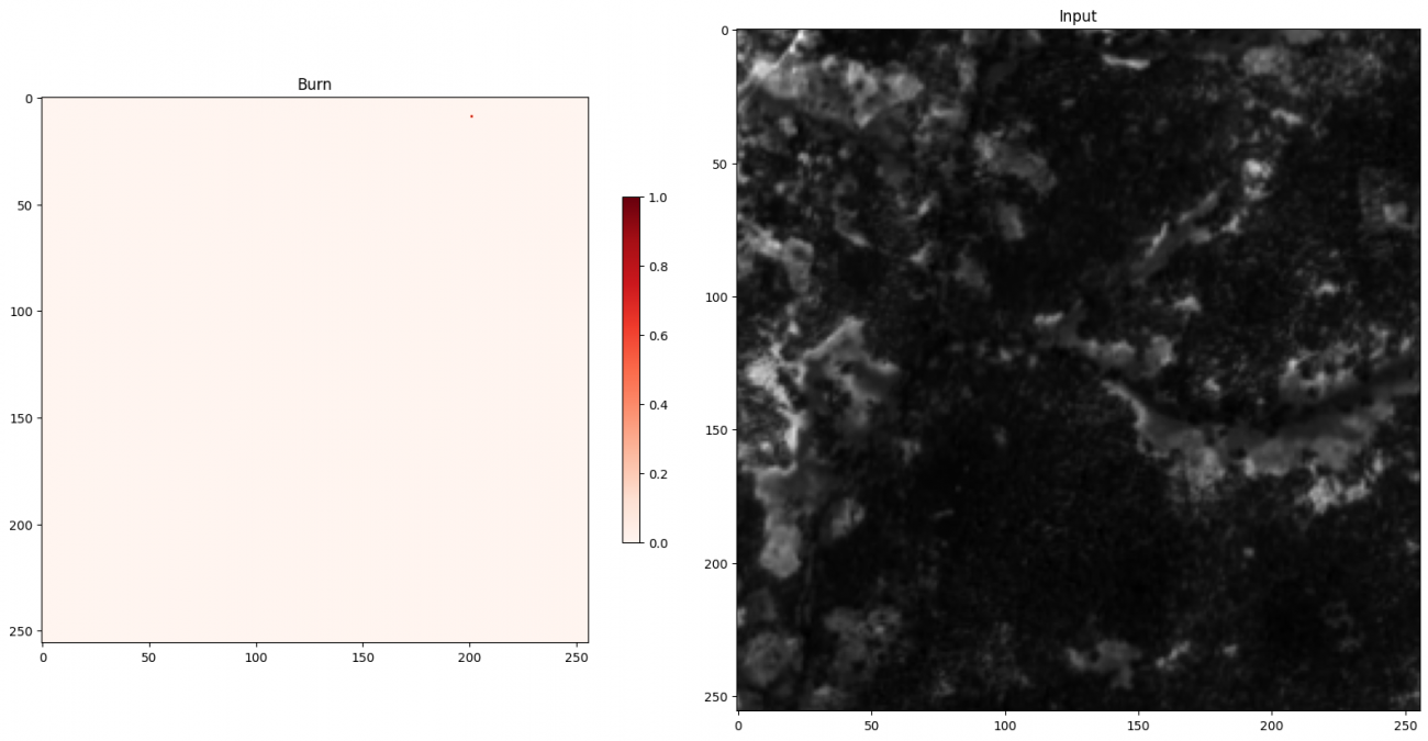
こちらも山火事はないのでほぼ 0 (真っ白)になっています。
最後に土壌被覆モデルです。
土壌被覆モデルの重みを取得します。
!wget https://huggingface.co/ibm-nasa-geospatial/Prithvi-100M-multi-temporal-crop-classification/resolve/main/multi_temporal_crop_classification_Prithvi_100M.pth -P ./pretrain/同様に前処理をします。
import tifffile
import cv2
import numpy as np

img = tifffile.imread('../../sample/ROIs1158_spring_s2/s2_1/ROIs1158_spring_s2_1_p30.tif')
print(img.shape, img.dtype)

# 13 --> 6
img = cv2.resize(img, (224, 224), interpolation=cv2.INTER_CUBIC)
img_band = np.stack([
    img[:, :, 1], img[:, :, 2], img[:, :, 3], # RGB
    img[:, :, 7], img[:, :, 11], img[:, :, 12],
    img[:, :, 1], img[:, :, 2], img[:, :, 3], # RGB
    img[:, :, 7], img[:, :, 11], img[:, :, 12],
    img[:, :, 1], img[:, :, 2], img[:, :, 3], # RGB
    img[:, :, 7], img[:, :, 11], img[:, :, 12],
    ],
    axis=0)

print(img_band.shape, img_band.dtype)

# save as tif
tifffile.imwrite('input/crop/ROIs1158_spring_s2_1_p30_crop.tif', img_band)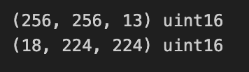
同じく設定を変更します。
configs/multi_temporal_crop_classification.pyのファイルの以下を編集します。
- channel_last=True
+ channel_last=False
土壌分類の推論をします。
!python model_inference.py -config configs/multi_temporal_crop_classification.py \
    -ckpt ../pretrain/multi_temporal_crop_classification_Prithvi_100M.pth \
    -input input/crop/ \
    -output output/crop/ -input_type tif -bands "[0,1,2,3,4,5]"
分類クラスは以下のようになっています。
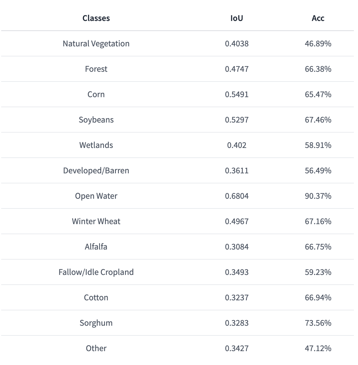
0:天然植生
1:森
2:トウモロコシ
3:大豆
4:湿地
5:開拓地
6:広範囲水域
7:麦
8:ウマゴヤシ
9:綿
10:モロコシ
11:その他
分類結果を可視化します。
PATH_OUT = f'output/crop/ROIs1158_spring_s2_1_p30_crop_pred.tif'

import matplotlib.pyplot as plt
pred_t0 = tifffile.imread(PATH_OUT)
print(pred_t0.shape)

# plot image
plt.figure(figsize=(16, 8))
plt.subplot(1, 2, 1)
plt.title('Crop')
plt.imshow(pred_t0, cmap='Set3', vmin=0, vmax=12)
plt.colorbar(shrink=0.5)

plt.subplot(1, 2, 2)
plt.title('Input')
plt.imshow(img_band[-1], cmap='gray')

# off grid
plt.tight_layout()
plt.grid(False)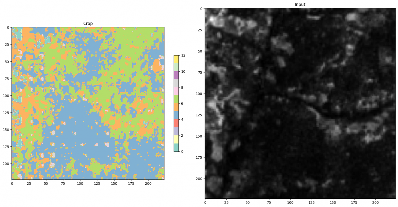
森っぽいと思っていましたが、開拓地や湿地などと予測されています。
凡例はクラス番号ごとに画像の右にあるスケールに記載されています。
Data Fusion
基盤モデルの時にも融合という言葉が出てきたように、複数の衛星画像を融合して使う「Data Fusion」という言葉が学会や論文でも散見されるようになりました。異なる衛星や異なるセンサーでの特徴を、違うモデルに移植するなどのソフトウェアでの取り組みになります。
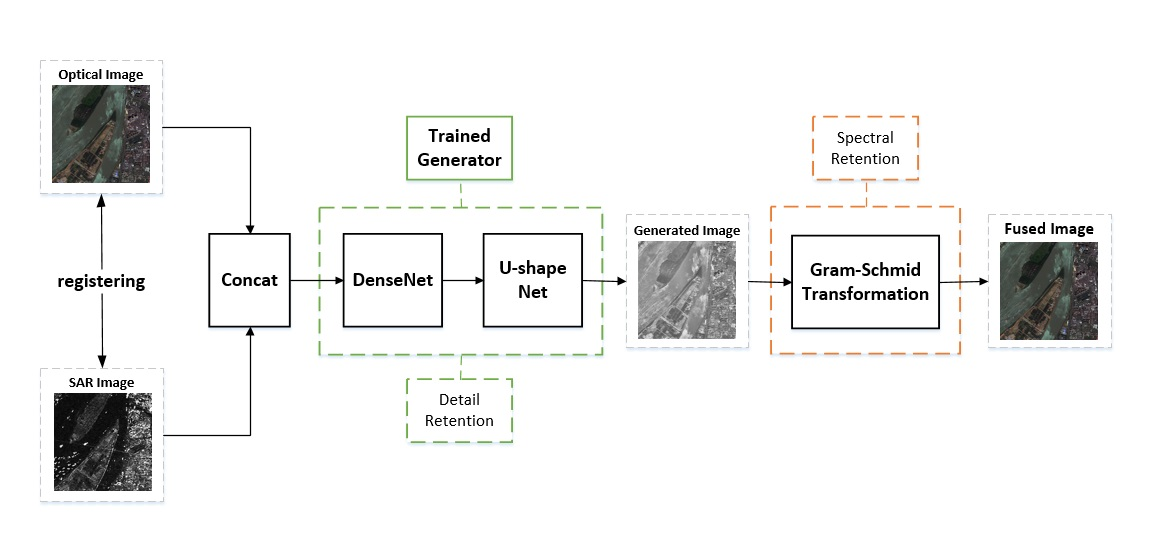
グラムシュミット変換を用いて独立した特徴量を上手に合成する手法の提案です。
Source : https://www.sciencedirect.com/science/article/pii/S1569843222000206
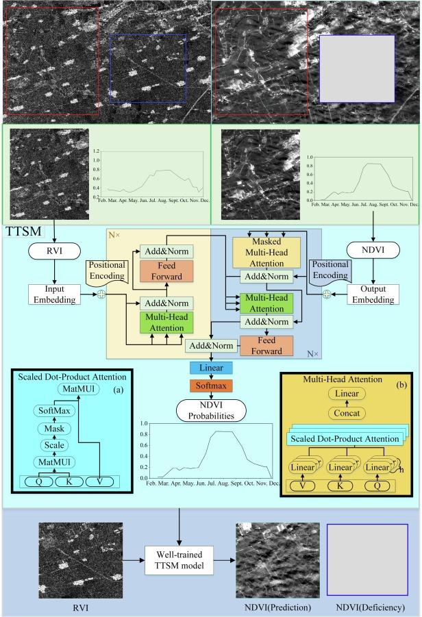
光学衛星とSAR衛星での NDVI と RVI を Transfomer のアテンション機構により欠落した光学の NDVI を補完するような手法の提案です。
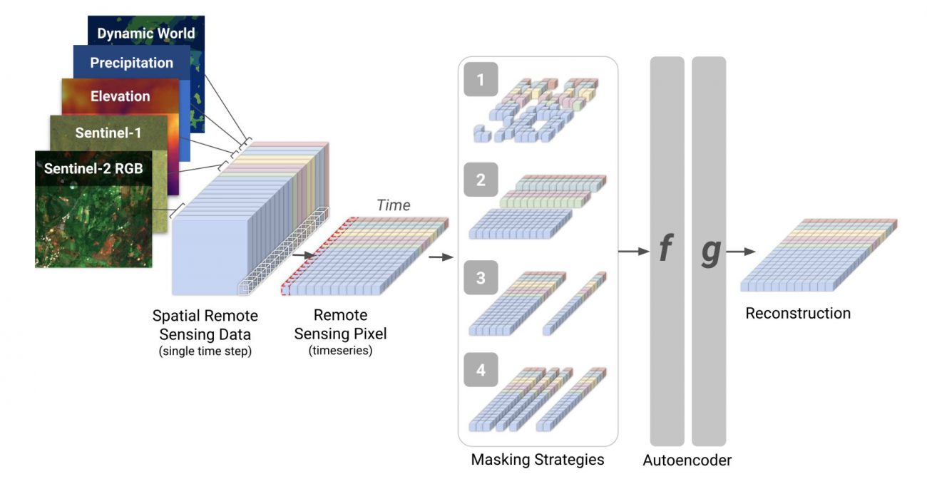
複数の衛星センサーのデータと地理空間データを同時に Transformer モデルに学習させることで一般表現を獲得できるという手法の提案です。
再構成させることによってパッチで細分化されている特徴の理解を狙った方法だと思います。言語モデル(LLMなど)は Masked Language Model (MLM) の事前学習を行うものが多く、それを画像に取り入れた方法です。MAE (Masked Auto Encoder) も同様の手法になります。
Githubにコードが公開されています。
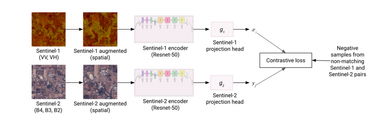
同一の場所を光学衛星とSAR衛星で撮像して、それぞれを対象それぞれのモデルに学習させます。対照学習(Contrastive Learning)によって同じエリアは同一の場所であるように教え込まれます。
データを融合するだけでなく、その特徴をモデルに蒸留・埋め込むような手法の提案です。これによって事前学習されたモデルは光学モデルだが、SARの得意な部分を、SARモデルだが光学の得意な部分の精度が上がるように報告されています。
Data Fusion についての実装はないですがこれからの衛星データの流れの一つなのでぜひ、念頭に入れておいても良いかもしれません。
Github
コードは宙畑のGithubで公開しています。
環境構築は以下です。
docker compose -f compose_foundation.yml up -dまとめ
最新の衛星データの取り組みを紹介しました。衛星ハードの進歩と共に衛星データのソフトも日々進化しています。気になるものがあればぜひ、触ってみてください。
宙畑でも、出来る限り新しいトピックは注視してこれはというものは記事でご紹介できればと考えています。ぜひ、このトピックが気になる!というものがあれば宙畑までご連絡いただけますと幸いです。
