宙畑では、たびたび桜の開花に関する衛星データの記事を公開しています。

■過去の衛星データ×桜に関する記事

有名な場所に行けば間違いなく桜を楽しめますが、有名な場所は人も多く、できれば穴場を探したいもの。そこで、もともとは衛星データから桜は見えるのか!?と思って始めたのですが、無料の衛星データから細かく桜の木1本1本を探すのを至難の技でした。

そして、「もっといい場所が見たい」「思ったより見づらい」など現地に行ってみないとわからないことが多いのも事実。そこで考えたのが高解像度の衛星データを活用して桜を自動で検知しよう！という試みです。

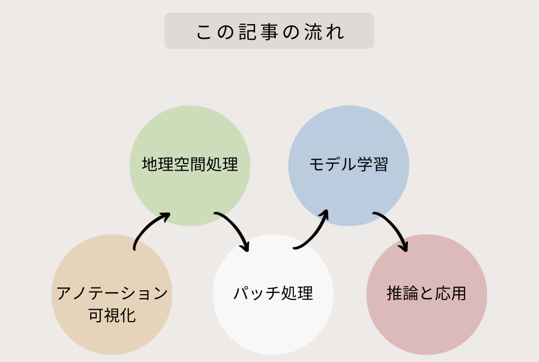
今回は以下のような流れで、自動的に探して桜の見え方を検証する方法を解説します。

アノテーションの方法については、事前に宙畑編集部で行ったものを利用しますので、ここでは解説を割愛いたします。アノテーションのやり方について興味がある方は「衛星データのアノテーション方法～QGISでのポリゴン作成と利用する際の注意点～」をご覧ください。

桜のポリゴンを可視化

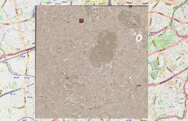
まずはアノテーションしたデータをQGISで地理空間で可視化します。

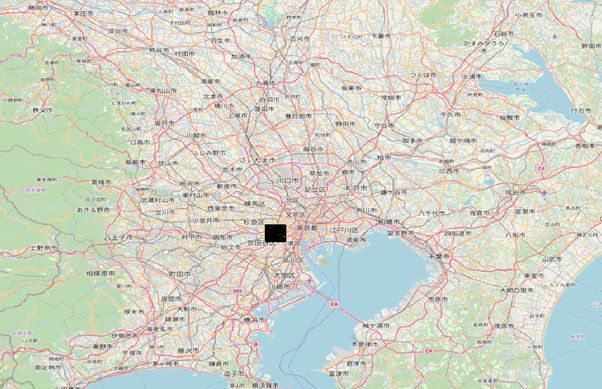
場所は東京都の渋谷区周辺です。

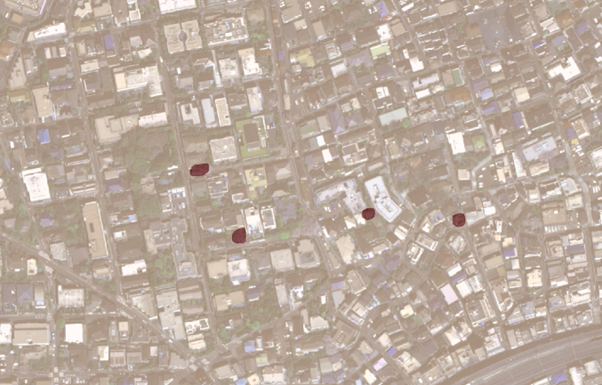
近くで見てみましょう。

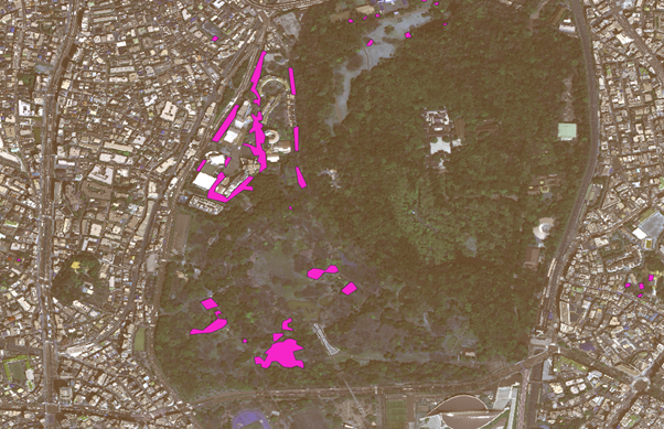
代々木公園でポリゴン処理した場所を比較します。

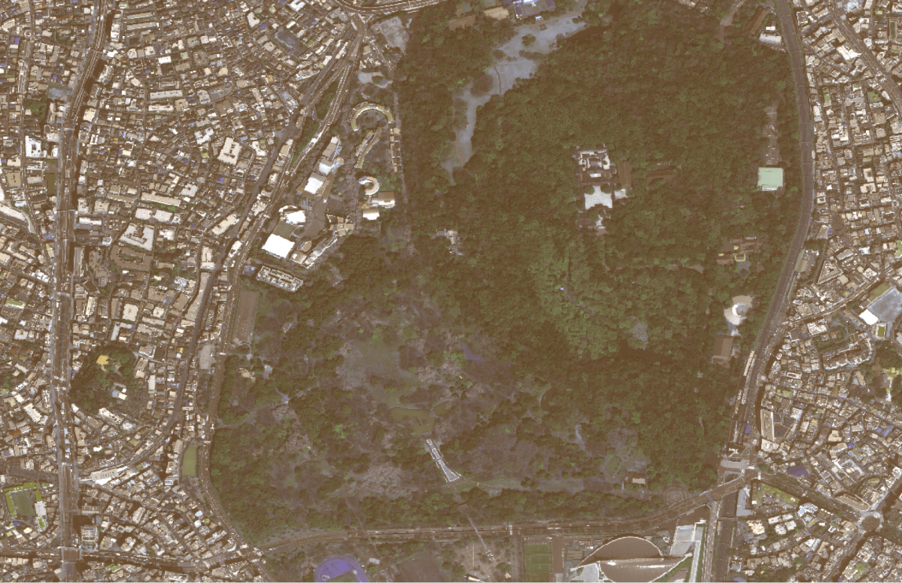
正しくアノテーションができていそうですね。

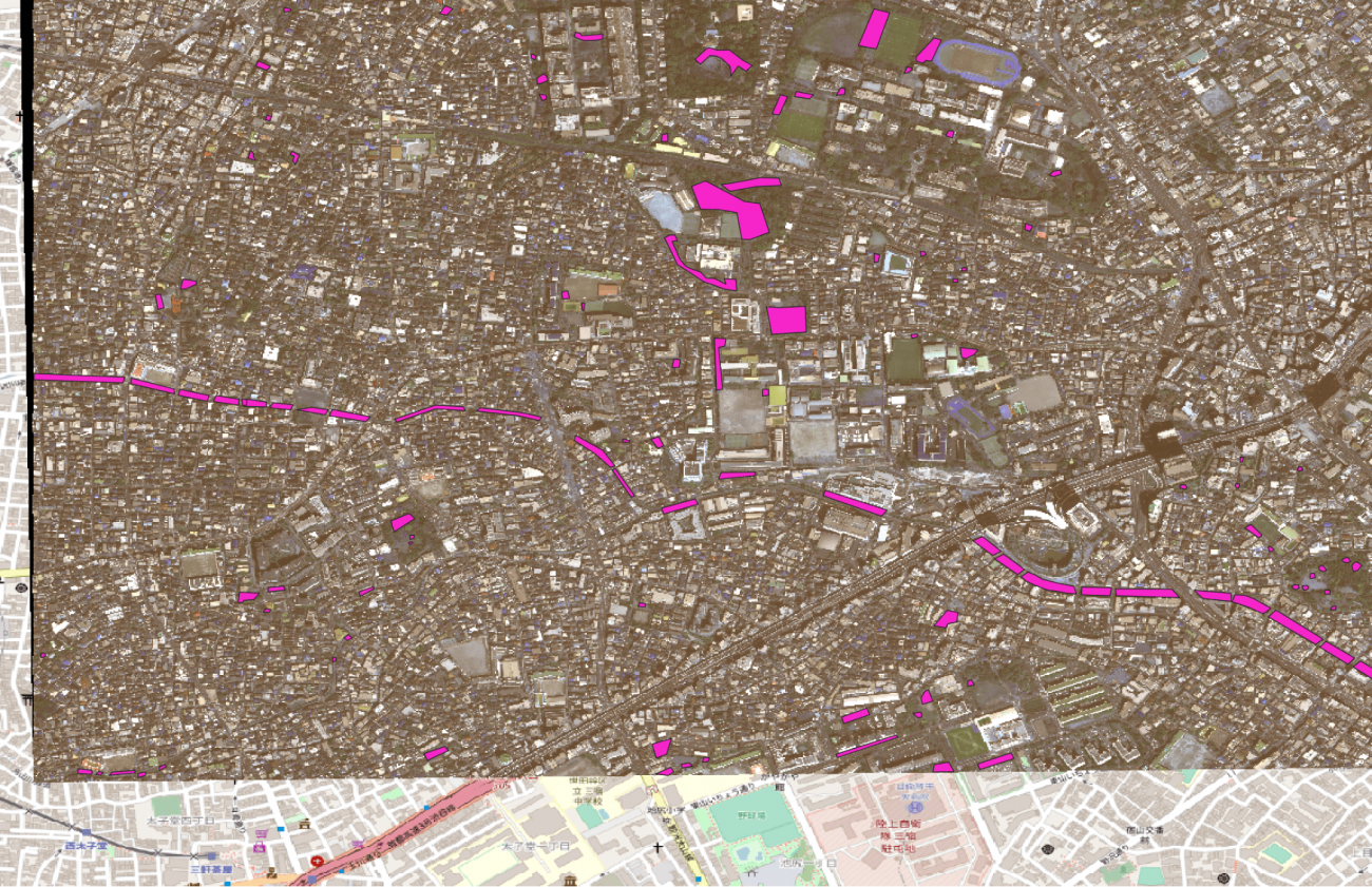
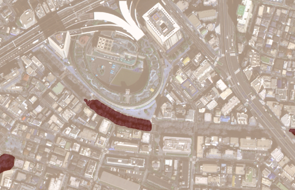
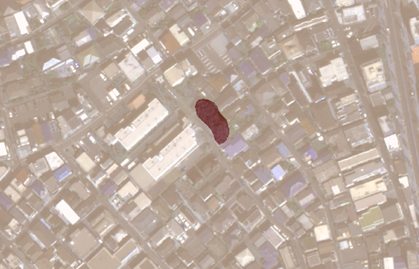
目黒川の桜もアノテーションしてみましたが、こうして俯瞰して見てみるとかなり長い距離で桜が並んでいることがわかります。
このように実際に体感したことある感覚と地図上での規模を理解するのには桜は身近なとても良い題材ですね。

地理空間データの変換

続いては、地理空間データの変換です。地理空間の環境構築では難儀した人は多いでしょう。今回は以下の宙畑の記事を利用して簡単に作成します。

宙畑では記事で紹介したコードをGithubにまとめていますので、ぜひ参考にしていただけますと幸いです。

学習環境も含めて以下のDocker環境で揃います

docker compose up -d

まずは全体を True color で可視化します。

c_s_min = [300, 300, 190]
c_s_max = [600, 900, 730]

imgs = []

for _c in range(3):
    _img = np.clip(img[_c, :, :], c_s_min[_c], c_s_max[_c])
    _img = (_img - c_s_min[_c]) / c_s_max[_c]    
    imgs.append(_img)

imgs_true = (np.stack(imgs, axis=2) * 255).astype(np.uint8)[:,:,::-1]

plt.figure(figsize=(12, 10))
plt.title('True Color')
plt.imshow(imgs_true)
plt.show();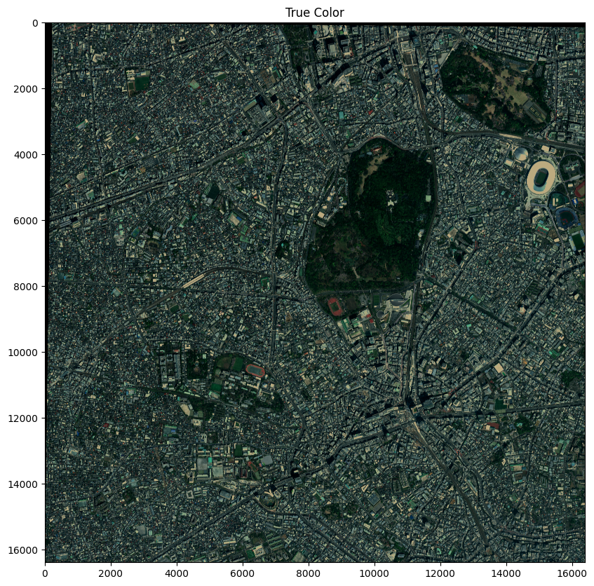

次に False Color（植生を強く反射する近赤外（NIR）を赤に配色し、赤が濃いところほど植物が多いことを示したもの）を可視化します。

c_s_min = [300, 300, 190]
c_s_max = [600, 900, 730]

imgs = []

for _c in range(3):
    _img = np.clip(img[_c+1, :, :], c_s_min[_c], c_s_max[_c])
    _img = (_img - c_s_min[_c]) / c_s_max[_c]
    
    imgs.append(_img)

imgs_false = (np.stack(imgs, axis=2) * 255).astype(np.uint8)[:,:,::-1]

plt.figure(figsize=(12, 10))
plt.title('False Color')
plt.imshow(imgs_false)
plt.show();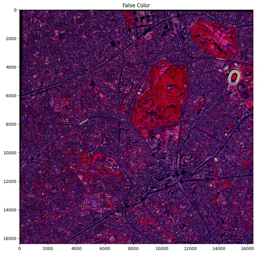

False Colorなど、波長を用いた衛星画像解析については以下の記事をご覧ください。

続いて、アノテーションを可視化します。

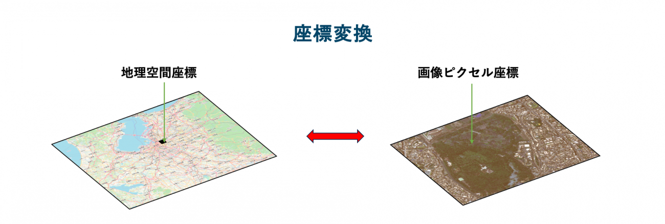
ここで注意すべきことがあります。 GeoJson形式では地理空間座標となっています。これを画像のピクセルでの座標に投影して変換しなければなりません。

def geo2pixel(ts, ds):
    """
    Inverse GeoCode Function
    """

    affine = ds.transform
    n = np.array(affine)
    a, b, xoff, d, e, yoff  = n[0],n[1], n[2], n[3], n[4], n[5]
    
    ret = []
    for t in ts:
        x, y = t[0], t[1]
        mat = np.array([[a, b], [d, e]]).astype(np.float32)
        inv = np.linalg.inv(mat)
       
        xp = (x - xoff) *inv[0][0] +  (y-yoff) *inv[0][1] 
        yp = (x - xoff) *inv[1][0] +  (y-yoff)*inv[1][1] 
        ret.append([xp, yp])

    return ret

こちらの関数で内部のCRS（Coordinate Reference Syste（Coordinate Reference System）と言って地理空間の定義座標の逆行列からピクセル座標に変換します。

CRS についてはこちらが詳しいです。

convert_ano_to_json(
    train_ano_json_path=DATASET_ROOT + 'sakura_segs.json', 
    output_dir=DATASET_ROOT, 
    dataset_dir=DATASET_ROOT, 
    random_seed=417
)

加えて、同時に機械学習でよく使用される COCO 形式に変換します。

COCO (Common Object in Context) とは、Microsoft が公開したデータセットの形式の１つです。主に物体検知で使用されています。

COCO APIというライブラリーも公開されています。

これを利用して簡易的に確認します。

coco = COCO(DATASET_ROOT + f'train_scale{SCALE}_segs.json')
print()
cats = coco.loadCats(coco.getCatIds())
nms = [cat['name'] for cat in cats]
print('Sorabatake COCO sakura categories: \n{}\n'.format(' '.join(nms)))

画像ごとのメタデータを確認します。

catIds = coco.getCatIds(catNms=['sakura']);
imgIds = coco.getImgIds(catIds=catIds);
image_idx = 1
imgIds = coco.getImgIds(imgIds=[image_idx])
img_info = coco.loadImgs(imgIds[np.random.randint(0,len(imgIds))])[0]
print(img_info)
os.makedirs(OUTPUT, exist_ok=True)

では、アノテーションを可視化します。

plt.figure(figsize=(24, 20), facecolor='white')
plt.title('Sakura annotation')
plt.imshow(np.zeros((round(img_info['height']), round(img_info['width']), 3)));
annIds = coco.getAnnIds(imgIds=img_info['id'], catIds=catIds, iscrowd=None)
anns = coco.loadAnns(annIds)
coco.showAnns(anns, draw_bbox=True)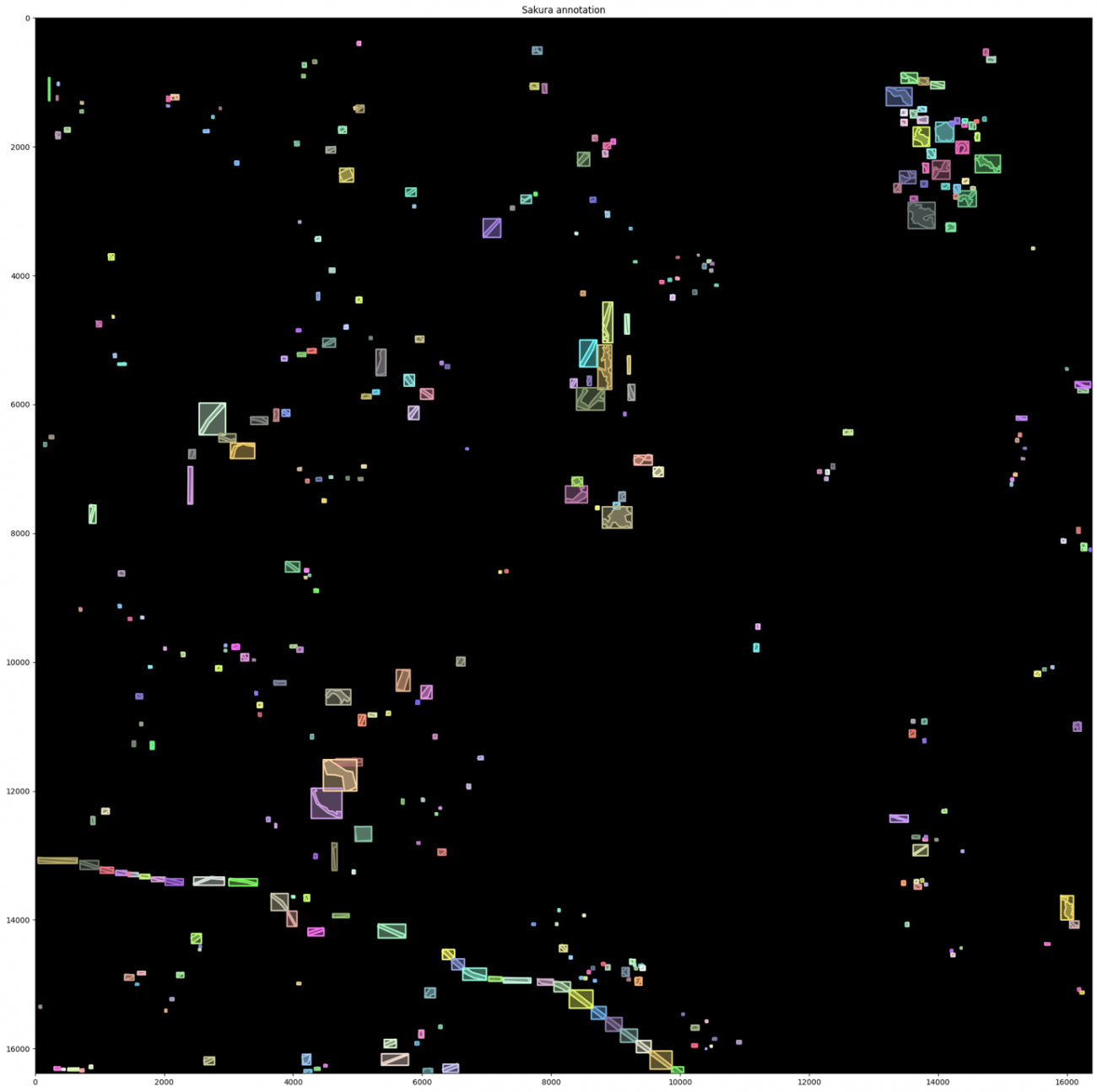

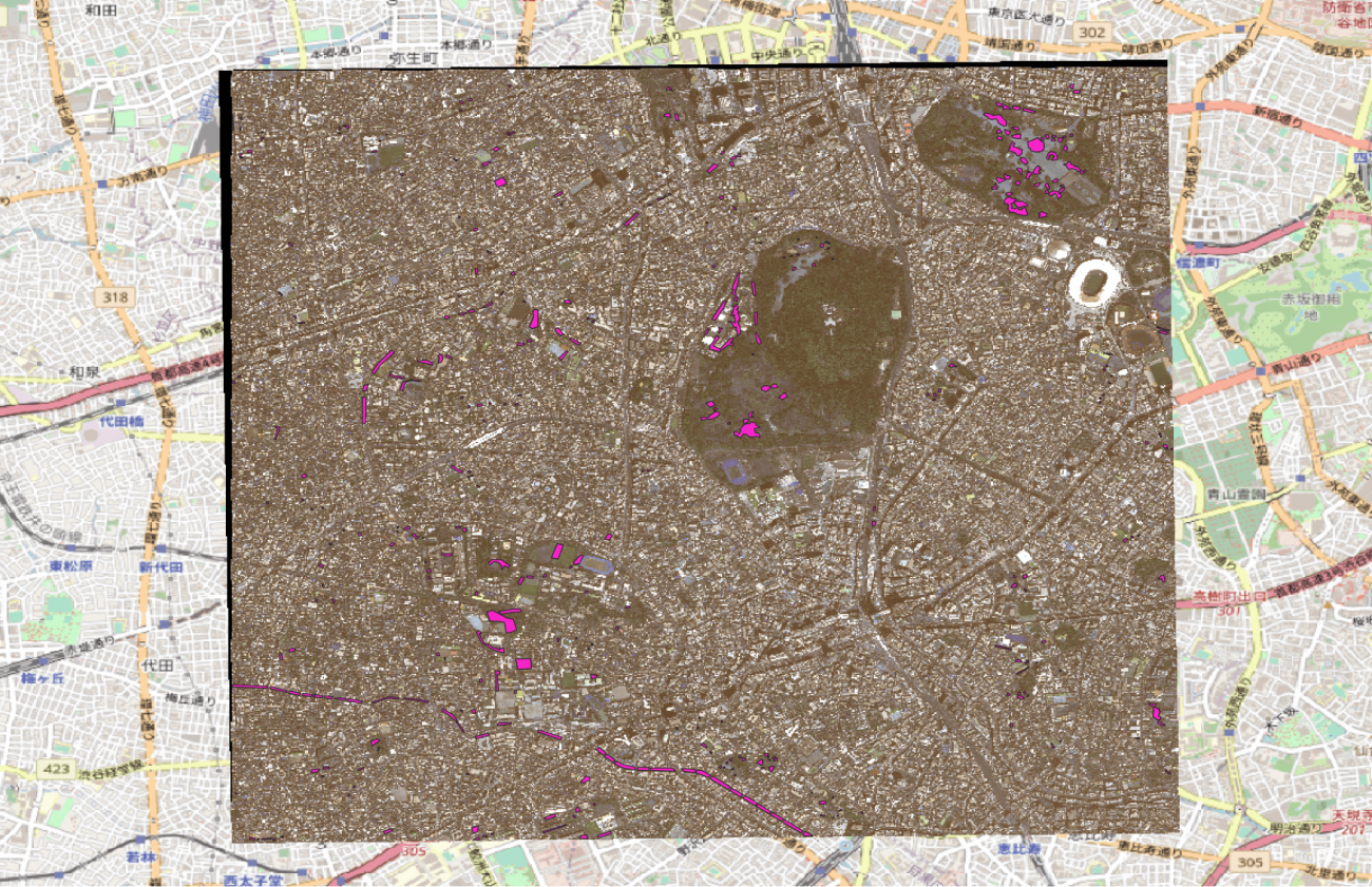
True Color に重畳して可視化します。

plt.figure(figsize=(24, 20), facecolor='white')
plt.title('True Color with sakura annotation')
plt.imshow(imgs_true);
annIds = coco.getAnnIds(imgIds=img_info['id'], catIds=catIds, iscrowd=None)
anns = coco.loadAnns(annIds)
coco.showAnns(anns, draw_bbox=True)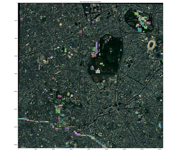

False Color に重畳して可視化します。

plt.figure(figsize=(24, 20), facecolor='white')
plt.title('False Color with sakura annotation')
plt.imshow(imgs_false, alpha=0.75);
annIds = coco.getAnnIds(imgIds=img_info['id'], catIds=catIds, iscrowd=None)
anns = coco.loadAnns(annIds)
coco.showAnns(anns, draw_bbox=True)

先ほど確認した目黒川などの目印になるような場所で確認するとずれているかも確認しやすいでしょう。

パッチによる切り取り

衛星画像は非常に大きく、今回の場合でも 16384 x 16384 の画像サイズがあります。

機械学習をするには、物理的なメモリの制約があるのでパッチごとの画像に切り分けていきます。

このように処理することをパッチ化やスライディングウィンドウ処理とも言います。処理画像を見ていただく方がわかりやすいと思います。

今回はSAHI (Slicing Aided Hyper Inference) というライブリーを使用します。

パッチ処理の設定をします。

class CFG(object):
    
    def __init__(self,):
        self.image_dir: str = DATASET_ROOT
        self.coco_annotation_file_path = f'{DATASET_ROOT}train_scale{SCALE}_segs.json'
        
        self.ignore_negative_samples: bool = True
        self.slice_height: int = 640
        self.slice_width: int = 640
        self.overlap_height_ratio: float = 0.0
        self.overlap_width_ratio: float = 0.0
        self.min_area_ratio: float = 1
        self.verbose:bool = False
        self.out_ext:str = '.tif'
        
        self.output_dir = f'{DATASET_ROOT}train_scale{SCALE}_h{self.slice_height}_w{self.slice_width}_oh{self.overlap_height_ratio}_ow{self.overlap_width_ratio}_min{self.min_area_ratio}_segs/'
            
        self.output_coco_annotation_file_name = f"_sahi"
        
pprint(CFG().__dict__)

切り取っていきます。正しく切り取れたかを可視化します。

coco_dict, coco_path = slice_coco(
    **{k:v for k, v in CFG().__dict__.items() if not '__' in k}
)
print(coco_path)

c_s_min = [300, 300, 190, 190]
c_s_max = [600, 900, 730, 730]

catIds = coco.getCatIds(catNms=['sakura']);
imgIds = coco.getImgIds(catIds=catIds);
for image_idx in range(1, 6):
    imgIds = coco.getImgIds(imgIds=[image_idx])
    img_info = coco.loadImgs(imgIds[0])[0]
    print(img_info)
    
    I = tifffile.imread(f'{PATH_IMG}/{img_info["file_name"]}')

    imgs = []
    for _c in range(4):
        _img = np.clip(I[_c, :, :], c_s_min[_c], c_s_max[_c])
        _img = (_img - c_s_min[_c]) / c_s_max[_c]
        imgs.append(_img)

    imgs_false = (np.stack(imgs[1:], axis=2) * 255).astype(np.uint8)[:,:,::-1]
    imgs_true = (np.stack(imgs[:3], axis=2) * 255).astype(np.uint8)[:,:,::-1]

    plt.figure(figsize=(16, 16), facecolor='white')
    plt.title('Sample Patch True Sakura Annotation', fontsize=20, fontweight='bold')
    plt.imshow(imgs_true);
    annIds = coco.getAnnIds(imgIds=img_info['id'], catIds=catIds, iscrowd=None)
    anns = coco.loadAnns(annIds)
    coco.showAnns(anns)
    os.makedirs(OUTPUT, exist_ok=True)
    plt.tight_layout()
    plt.savefig(f'{OUTPUT}visualize_coco_sakura_sample-patch_true_I{image_idx}.png', format='png')
    plt.show();
    
    plt.figure(figsize=(16, 16), facecolor='white')
    plt.title('Sample Patch False Sakura Annotation', fontsize=20, fontweight='bold')
    plt.imshow(imgs_false);
    coco.showAnns(anns)
    os.makedirs(OUTPUT, exist_ok=True)
    plt.tight_layout()
    plt.savefig(f'{OUTPUT}visualize_coco_sakura_sample-patch_false_I{image_idx}.png', format='png')
    plt.show();
    
    plt.clf()
    plt.close()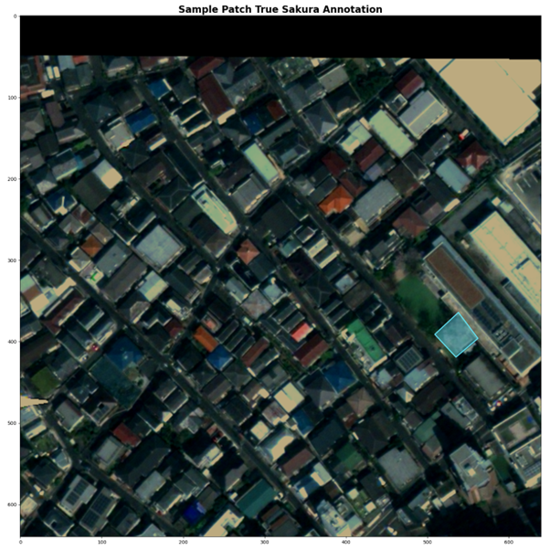

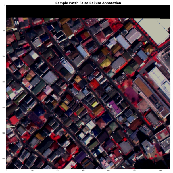
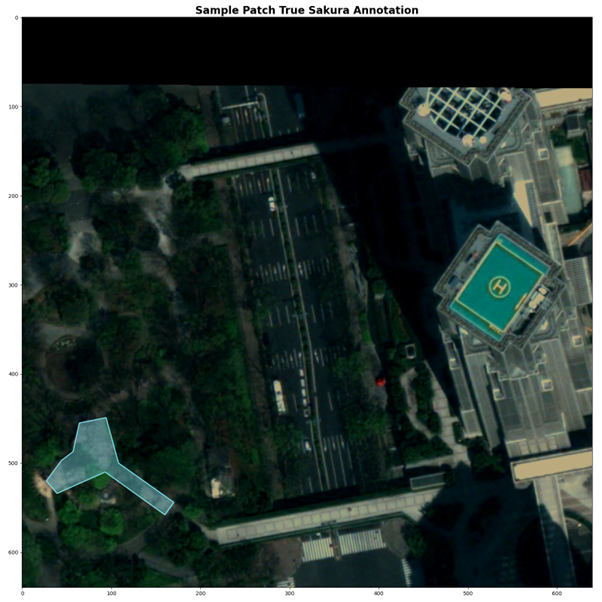
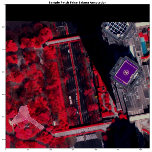
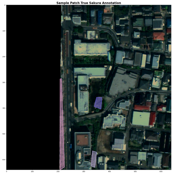
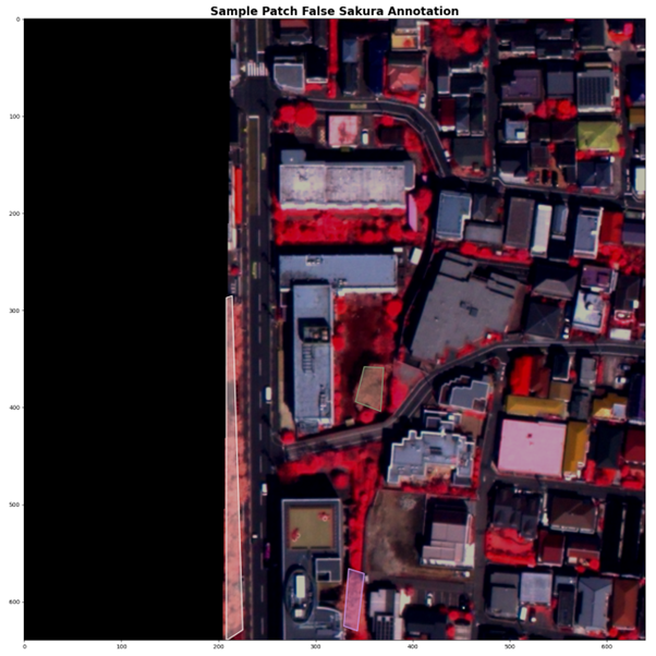
地理空間情報のアノテーションが画像内でのピクセル情報にピッタリと合っていますね。位置情報を精密に取得し、変換できるからこその処理ですね。

ここで以下のエラーが出ることがあります。

GEOSException: TopologyException: Input geom 0 is invalid: Self-intersection at 13714.467576791809 2958.3242320819113

これは SAHI ライブラリー内部で shapely というポリゴン処理をしているのですが、データの中に無効なポリゴンが含まれているからです。無効なポリゴンとは、自己交差が主な原因です。解決する方法は「geom 0 is INVALID: Self-intersection 自己交差エラーとその回避」を参考にしてください。

自動予測のモデル開発

では、いよいよ自動予測のモデル開発に進みましょう。今回は MMdetection を使用します。

基本的な処理は同じくMMdetection を使用した「駐車場に停まっている車両の検知精度アップ？ 衛星データによる車両の回転検知とその実装方法」の中で記載してありますので重複部分は割愛します。

大きなモデルは同じですが、今回は物体検知と共にセグメンテーションを行う、インスタンスセグメンテーションというタスクで桜の領域をポリゴンのような形で検知します。

さらに、Maxarの画像は4バンドの画像なので通常はRGBの画像モデルを拡張します。モデルはRTMDetを使用します。

RTMDet の CSPneXt というバックボーンの入力を変更します。

@MODELS.register_module()
class CSPNeXt(BaseModule):
    """CSPNeXt backbone used in RTMDet.

    Args:
        arch (str): Architecture of CSPNeXt, from {P5, P6}.
            Defaults to P5.
        expand_ratio (float): Ratio to adjust the number of channels of the
            hidden layer. Defaults to 0.5.
        deepen_factor (float): Depth multiplier, multiply number of
            blocks in CSP layer by this amount. Defaults to 1.0.
        widen_factor (float): Width multiplier, multiply number of
            channels in each layer by this amount. Defaults to 1.0.
        out_indices (Sequence[int]): Output from which stages.
            Defaults to (2, 3, 4).
        frozen_stages (int): Stages to be frozen (stop grad and set eval
            mode). -1 means not freezing any parameters. Defaults to -1.
        use_depthwise (bool): Whether to use depthwise separable convolution.
            Defaults to False.
        arch_ovewrite (list): Overwrite default arch settings.
            Defaults to None.
        spp_kernel_sizes: (tuple[int]): Sequential of kernel sizes of SPP
            layers. Defaults to (5, 9, 13).
        channel_attention (bool): Whether to add channel attention in each
            stage. Defaults to True.
        conv_cfg (:obj:`ConfigDict` or dict, optional): Config dict for
            convolution layer. Defaults to None.
        norm_cfg (:obj:`ConfigDict` or dict): Dictionary to construct and
            config norm layer. Defaults to dict(type='BN', requires_grad=True).
        act_cfg (:obj:`ConfigDict` or dict): Config dict for activation layer.
            Defaults to dict(type='SiLU').
        norm_eval (bool): Whether to set norm layers to eval mode, namely,
            freeze running stats (mean and var). Note: Effect on Batch Norm
            and its variants only.
        init_cfg (:obj:`ConfigDict` or dict or list[dict] or
            list[:obj:`ConfigDict`]): Initialization config dict.
    """
    # From left to right:
    # in_channels, out_channels, num_blocks, add_identity, use_spp
    arch_settings = {
        'P5': [[64, 128, 3, True, False], [128, 256, 6, True, False],
               [256, 512, 6, True, False], [512, 1024, 3, False, True]],
        'P6': [[64, 128, 3, True, False], [128, 256, 6, True, False],
               [256, 512, 6, True, False], [512, 768, 3, True, False],
               [768, 1024, 3, False, True]]
    }

    def __init__(
        self,
        arch: str = 'P5',
        stem_channels: int=4,
        deepen_factor: float = 1.0,
        widen_factor: float = 1.0,
        out_indices: Sequence[int] = (2, 3, 4),
        frozen_stages: int = -1,
        use_depthwise: bool = False,
        expand_ratio: float = 0.5,
        arch_ovewrite: dict = None,
        spp_kernel_sizes: Sequence[int] = (5, 9, 13),
        channel_attention: bool = True,
        conv_cfg: OptConfigType = None,
        norm_cfg: ConfigType = dict(type='BN', momentum=0.03, eps=0.001),
        act_cfg: ConfigType = dict(type='SiLU'),
        norm_eval: bool = False,
        init_cfg: OptMultiConfig = dict(
            type='Kaiming',
            layer='Conv2d',
            a=math.sqrt(5),
            distribution='uniform',
            mode='fan_in',
            nonlinearity='leaky_relu')
    ) -> None:
        super().__init__(init_cfg=init_cfg)
        arch_setting = self.arch_settings[arch]
        if arch_ovewrite:
            arch_setting = arch_ovewrite
        assert set(out_indices).issubset(
            i for i in range(len(arch_setting) + 1))
        if frozen_stages not in range(-1, len(arch_setting) + 1):
            raise ValueError('frozen_stages must be in range(-1, '
                             'len(arch_setting) + 1). But received '
                             f'{frozen_stages}')

        self.out_indices = out_indices
        self.frozen_stages = frozen_stages
        self.use_depthwise = use_depthwise
        self.norm_eval = norm_eval
        conv = DepthwiseSeparableConvModule if use_depthwise else ConvModule
        self.stem = nn.Sequential(
            ConvModule(
                stem_channels,
                int(arch_setting[0][0] * widen_factor // 2),
                3,
                padding=1,
                stride=2,
                norm_cfg=norm_cfg,
                act_cfg=act_cfg),
            ConvModule(
                int(arch_setting[0][0] * widen_factor // 2),
                int(arch_setting[0][0] * widen_factor // 2),
                3,
                padding=1,
                stride=1,
                norm_cfg=norm_cfg,
                act_cfg=act_cfg),
            ConvModule(
                int(arch_setting[0][0] * widen_factor // 2),
                int(arch_setting[0][0] * widen_factor),
                3,
                padding=1,
                stride=1,
                norm_cfg=norm_cfg,
                act_cfg=act_cfg))
        self.layers = ['stem']


        for i, (in_channels, out_channels, num_blocks, add_identity,
                use_spp) in enumerate(arch_setting):
            in_channels = int(in_channels * widen_factor)
            out_channels = int(out_channels * widen_factor)
            num_blocks = max(round(num_blocks * deepen_factor), 1)
            stage = []
            conv_layer = conv(
                in_channels,
                out_channels,
                3,
                stride=2,
                padding=1,
                conv_cfg=conv_cfg,
                norm_cfg=norm_cfg,
                act_cfg=act_cfg)
            stage.append(conv_layer)
            if use_spp:
                spp = SPPBottleneck(
                    out_channels,
                    out_channels,
                    kernel_sizes=spp_kernel_sizes,
                    conv_cfg=conv_cfg,
                    norm_cfg=norm_cfg,
                    act_cfg=act_cfg)
                stage.append(spp)
            csp_layer = CSPLayer(
                out_channels,
                out_channels,
                num_blocks=num_blocks,
                add_identity=add_identity,
                use_depthwise=use_depthwise,
                use_cspnext_block=True,
                expand_ratio=expand_ratio,
                channel_attention=channel_attention,
                conv_cfg=conv_cfg,
                norm_cfg=norm_cfg,
                act_cfg=act_cfg)
            stage.append(csp_layer)
            self.add_module(f'stage{i + 1}', nn.Sequential(*stage))
            self.layers.append(f'stage{i + 1}')

    def _freeze_stages(self) -> None:
        if self.frozen_stages >= 0:
            for i in range(self.frozen_stages + 1):
                m = getattr(self, self.layers[i])
                m.eval()
                for param in m.parameters():
                    param.requires_grad = False

    def train(self, mode=True) -> None:
        super().train(mode)
        self._freeze_stages()
        if mode and self.norm_eval:
            for m in self.modules():
                if isinstance(m, _BatchNorm):
                    m.eval()

    def forward(self, x: Tuple[Tensor, ...]) -> Tuple[Tensor, ...]:
        outs = []
        for i, layer_name in enumerate(self.layers):
            layer = getattr(self, layer_name)
            x = layer(x)
            if i in self.out_indices:
                outs.append(x)
        return tuple(outs)

加えて、Tiff 形式のファイルでマルチバンドに対応できるように IO を追加します。

@TRANSFORMS.register_module()
class LoadTifFromFile(BaseTransform):
    """Load Tiff file images.


    Required Keys:


    - img_path


    Modified Keys:


    - img
    - img_shape
    - ori_shape


    Args:
        to_float32 (bool): Whether to convert the loaded image to a float32
            numpy array. If set to False, the loaded image is an uint8 array.
            Defaults to False.
        file_client_args (dict): Arguments to instantiate the
            corresponding backend in mmdet <= 3.0.0rc6. Defaults to None.
        backend_args (dict, optional): Arguments to instantiate the
            corresponding backend in mmdet >= 3.0.0rc7. Defaults to None.
    """


    def __init__(
        self,
        to_float32: bool = False,
        file_client_args: dict = None,
        backend_args: dict = None,
    ) -> None:
        self.to_float32 = to_float32
        self.backend_args = backend_args
        if file_client_args is not None:
            raise RuntimeError(
                'The `file_client_args` is deprecated, '
                'please use `backend_args` instead, please refer to'
                'https://github.com/open-mmlab/mmdetection/blob/main/configs/_base_/datasets/coco_detection.py'  # noqa: E501
            )


    def transform(self, results: dict) -> dict:
        """Transform functions to load multiple images and get images meta
        information.


        Args:
            results (dict): Result dict from :obj:`mmdet.CustomDataset`.


        Returns:
            dict: The dict contains loaded images and meta information.
        """


        assert isinstance(results['img_path'], str)
        img = tifffile.imread(results['img_path'])
        
        # C, H, W -> H, W, C
        img = img.transpose(1, 2, 0)
        if self.to_float32:
            img = img.astype(np.float32)


        results['img'] = img
        results['img_shape'] = img.shape[:2]
        results['ori_shape'] = img.shape[:2]
        return results


    def __repr__(self):
        repr_str = (f'{self.__class__.__name__}('
                    f'to_float32={self.to_float32}, '
                    f'backend_args={self.backend_args})')
        return repr_str

では、学習していきます。

/opt/conda/bin/python /workspace/src/mmdetection/tools/train.py /workspace/src/cfg/rtmdet-l_ins.py

本記事では、精度よりは方法のご紹介をしたいので学習と検証データは同じにしています。

推論してデバッグのような作業をしていきます。

/opt/conda/bin/python /workspace/src/mmdetection/tools/test.py \
    work_dirs/rtmdet-l_ins/rtmdet-l_ins.py work_dirs/rtmdet-l_ins/epoch_50.pth  \
    --work-dir work_dirs/rtmdet-l_ins/inference/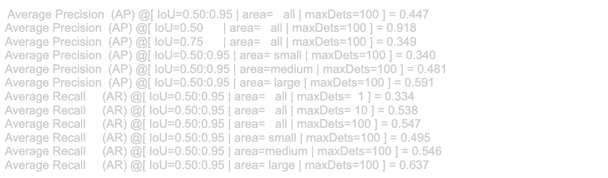

segm mAP50： 0.918 なので学習ができていそうですね。

予測領域ごとに見ていきます。

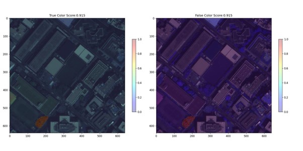
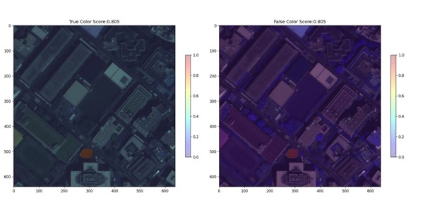
for res in results.pred_instances:
    for score, mask, label, bbox in zip(res.scores, res.masks, res.labels, res.bboxes):

        if score > THRESHOLD:
            COUNT += 1
            
            sc = score.cpu().numpy()
            
            mask = mask.cpu().numpy()
            img = img / img.max()
            
            plt.figure(figsize=(16, 8), dpi=120)
            plt.subplot(1, 2, 1)
            plt.title(f'True Color Score:{sc:.3f}')
            plt.imshow(img[:, :, :3])
            
            plt.imshow(mask, alpha=0.3, cmap='jet')
            plt.colorbar(shrink=0.5)
            
            plt.subplot(1, 2, 2)
            plt.title(f'False Color Score:{sc:.3f}')
            plt.imshow(img[:, :, 1:])
            
            plt.imshow(mask, alpha=0.3, cmap='jet')
            plt.colorbar(shrink=0.5,)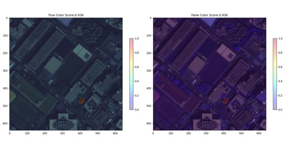

今度はスライディングウィンドウを行いながらパッチごとに予測します。

PATHS_TIF = glob("/workspace/sample/train_scale1_h640_w640_oh0.0_ow0.0_min1_segs/*.tif")
print(f'Num: {len(PATHS_TIF)}')

for PATH in tqdm(PATHS_TIF):
    
    img = tifffile.imread(PATH)
    img = img.astype(np.float32).transpose(1, 2, 0)
    
    if img.shape[:2] != (640, 640):
        continue

    results = inference_detector(model=model, imgs=img)
    
    pred = np.zeros((img.shape[:2]), dtype=np.float32)
    
    for res in results.pred_instances:
        for score, mask, label, bbox in zip(res.scores, res.masks, res.labels, res.bboxes):
            if score > THRESHOLD:
                mask = mask.cpu().numpy()
                pred += mask
    
    PATH_PRED = PATH.replace('.tif', '.png')
    
    pred = np.clip(pred * 255, a_max=255, a_min=0).astype(np.uint8)
    cv2.imwrite(PATH_PRED, pred)

元の画像に繋ぎ合わせて復元します。

PATHS_PATCH = glob('/workspace/sample/train_scale1_h640_w640_oh0.0_ow0.0_min1_segs/*.tif') 
print('Num Patch', len(PATHS_PATCH))

pred_org = np.zeros(img_org.shape[1:], dtype=np.uint8)
print(pred_org.shape)

for _P in tqdm(PATHS_PATCH, total=len(PATHS_PATCH)):
    ranges = _P.split('/')[-1].split('_')[-4:]
    crop_range_x_min = int(ranges[0])
    crop_range_x_max = int(ranges[2])
    crop_range_y_min = int(ranges[1])
    crop_range_y_max = int(ranges[3].replace('.tif', ''))
    
    pred = cv2.imread(_P.replace('.tif', '.png'), cv2.IMREAD_UNCHANGED)
    if pred is None:
        continue
    
    pred_org[crop_range_y_min:crop_range_y_max, crop_range_x_min:crop_range_x_max] = pred

plt.figure(figsize=(16, 16), facecolor='white')
plt.title('Original Size Predict', fontsize=20, fontweight='bold')
plt.imshow(pred_org);
plt.colorbar()

PATH_PRED_NO_GEO_TIF = '/workspace/sample/pred.tif'
tifffile.imwrite(PATH_PRED_NO_GEO_TIF, pred_org)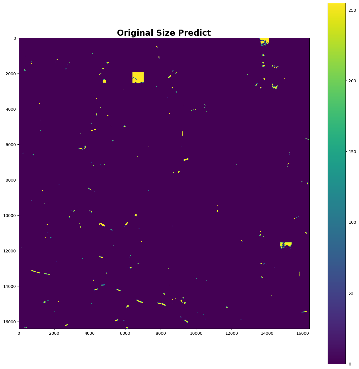

画像から地理空間処理

予測した領域の画像を地理空間上に投影します。

PATH_GEO = PATH_PRED_NO_GEO_TIF.replace('.tif', '_geo.tif')
with rasterio.open(PATH_PRED_NO_GEO_TIF) as geo_non:
    output_tiff = geo_non.read(1)

    with rasterio.open(PATH_ORG, 'r') as info:
        with rasterio.open(
                        PATH_GEO, 
                        'w', 
                        driver='GTiff', 
                        height=info.shape[0], 
                        width=info.shape[1], 
                        count=1, 
                        dtype=output_tiff.dtype, 
                        crs=info.crs, 
                        transform=info.transform) as out_info:

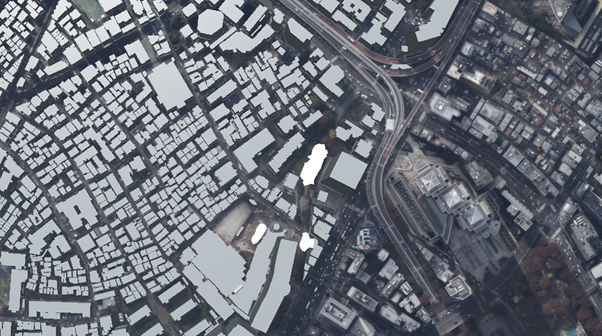
            out_info.write(output_tiff, 1)

QGISでAIの予測を可視化した結果が以下になります。

では、より細かく見ていきましょう。次の画像では、桜がしっかりと検知されているようですね。

一方で、以下の川沿いの画像のように見逃してしまっている箇所もあるようです。

しっかり検知できていますね。

ここまでで衛星データから桜の領域を自動でレコメンドしてくれるところまでが完了しました。

周囲の3D シミュレーション

最後に、桜の場所がわかるようになったので次は周囲の状況を調べていきます。

今回は、G空間センターの3D都市モデル 東京23区の建物データで周囲からどのように見えるのかを見ていきます。

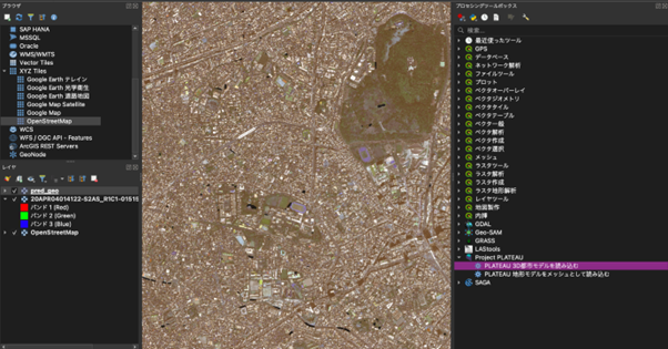
QGISのプラグインで3D都市モデルを読み込むためのツールが公開されているのでこちらを使用して読み込んでいきます。

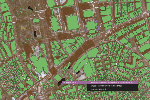
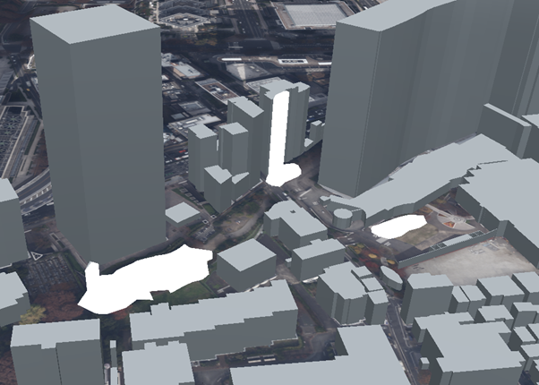
上の画像で緑になっている箇所が建物領域で、黒い部分が桜の予測領域です。

ここで、139.6927163,35.6844745の座標の桜をターゲットにしてみます。

ターゲットとした桜は、地上で花見スポットに適しているかは不明なので、建物の場所などを分かりやすくするため、３D上で確認します。

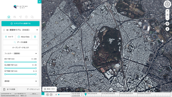
3D可視化はPlateau Viewを使用します。

例えば、先ほどの３D都市モデルで渋谷を投影しますと以下のようになります。

では、これまでに桜の予測を行った領域の座標を見てみましょう。

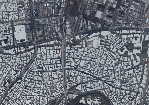
３D感がわかるように近づいて地表面から見てみます。

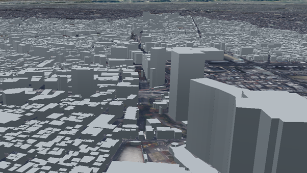
建物の高さがわかりますね。

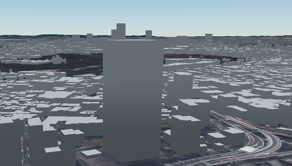
大きなビルの裏からだと見えそうにないですね。

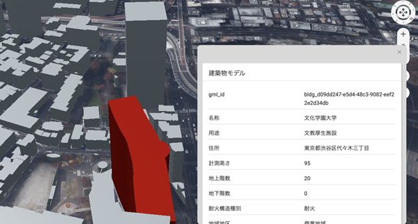
このビルを選択すると、建物の情報までわかります。すごい時代ですね!

そして、Plateau View ではオリジナルのファイルも投影することが可能です。

地理空間のベクターデータであれば読み込めるので、先ほど作成した桜の予測を行った場所のデータを変換して読み込ませていきましょう。

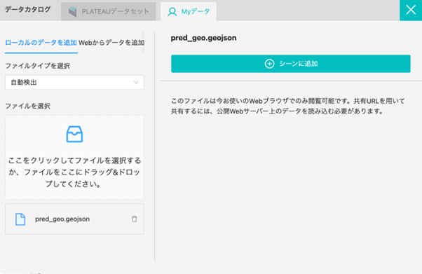
桜の領域が投影されました。例えば、以下の場所はいかがでしょうか。座標が重なっているとビルに乗っかっているように見えていますね。

別の角度からも見てみましょう。

動画で見てみるとさらに分かりやすいかもしれません。

詳しく見てみたところ、文化学園大学の敷地でした。ですので、お花見目的の公園としては利用できないようです。

このように自動化によってAIの推論は手軽で良いですが、最後は人間が判断して見極める必要があります。

コードと環境

本記事で使用したコードは以下で公開しています。ぜひ試してみたいという方は参考にしていただけますと幸いです。

Github: https://github.com/sorabatake/article_34076_cherry_blossom_detection

動作環境には Docker Compose + Nvidia Docker の環境が必要です。

mmdetection の環境構築は以下です。
docker compose up -d

前処理
https://github.com/sorabatake/article_34076_cherry_blossom_detection/blob/main/src/001_preprocess.ipynb

モデル学習
https://github.com/sorabatake/article_34076_cherry_blossom_detection/blob/main/src/002_train_mmdet.ipynb

モデル推論
https://github.com/sorabatake/article_34076_cherry_blossom_detection/blob/main/src/003_inference.ipynb

ジオコード
https://github.com/sorabatake/article_34076_cherry_blossom_detection/blob/main/src/004_geocode.ipynb

ファイルの配置は以下の記事に従っています。

まとめ

本記事では、桜を自動で予測するモデルの開発とそのための工夫ポイント、そして、自動予測した結果を3D上に表示して、どのような見え方をするのかのシミュレーションまで行いました。

興味を持たれた方はぜひご自身で衛星データのアノテーションから行い、実践してみてください。もしかしたら衛星データで家にいながら、近所のお花見の穴場が見つかるかもしれませんよ。