【コード付き】Sentinel-2の衛星画像から指定した範囲のタイムラプスを作成する
林野火災による被害が大きいオーストラリアを対象に、指定した期間の各月で最も被雲率の低い衛星画像を取得してタイムラプスを作成し、その被害状況を可視化する方法をご紹介します。
記事作成時から、Tellusからデータを検索・取得するAPIが変更になっております。該当箇所のコードについては、以下のリンクをご参照ください。
https://www.tellusxdp.com/ja/howtouse/access/traveler_api_20220310_
firstpart.html
2022年8月31日以降、Tellus OSでのデータの閲覧方法など使い方が一部変更になっております。新しいTellus OSの基本操作は以下のリンクをご参照ください。
https://www.tellusxdp.com/ja/howtouse/tellus_os/start_tellus_os.html
「【コード付き】Sentinelの衛星データをAPI経由で取得してみた」では指定した場所、期間で被雲率が最も低いSentinel-2の画像をAPIで引っ張ってくる方法についてご紹介しました。
今回は上記記事を応用し、指定した期間の各月で最も被雲率の低い衛星画像をAPIで取得し、タイムラプスを作成する方法をご紹介します。
1枚の画像として指定範囲を見るケースでも衛星画像の面白さはありますすが、同一地点を時系列に見ることで、より衛星の強味を活きます。
1. 対象エリアを選定
流れとしては過去記事と同様です。
import os
import numpy as np

from sentinelsat import SentinelAPI, read_geojson, geojson_to_wkt
import geopandas as gpd
import pandas as pd
import numpy as np
import matplotlib.pyplot as plt

from shapely.geometry import MultiPolygon, Polygon
import rasterio as rio
from rasterio.plot import show
import rasterio.mask
import fiona
import folium

#関心領域のポリゴン情報の取得
from IPython.display import HTML
HTML(r' width="960" height="480" src="https://www.keene.edu/campus/maps/tool/" frameborder="0">')
#実行する際には上記r'の次に<iframeの文字列をコピー・挿入して実行してください
#<は半角に変更してください

#上記にて取得した地理情報をコピペする
AREA =  [
      [
        150.3934479,
        -34.2354585
      ],
      [
        150.3925323,
        -34.3063876
      ],
      [
        150.5703735,
        -34.3064821
      ],
      [
        150.5707169,
        -34.23508
      ],
      [
        150.3934479,
        -34.2354585
      ]
    ]
ところで、関心領域のポリゴン情報の取得した際に、おや?と思った方もいるかもしれません。
具体的には、ポリゴンを取得した際に、緯度の数字は気にならないものの、経度がおかしいと思われた方もいたのではないでしょうか?
例えば、同じ領域でポリゴンを作成したはずなのに、下記のようになっていたり……。
[
        -210.0695801,
        -34.6535446
      ],
      [
        -210.0613403,
        -34.8814248
      ],
      [
        -209.6768188,
        -34.8971952
      ],
      [
        -209.6740723,
        -34.6648406
      ],
      [
        -210.0695801,
        -34.6535446
      ]
これは利用したツールの仕様上致し方のないところなのですが、右に移動すればするほど経度は360度ずつ加算され、左に移動すれば減算されていきます。
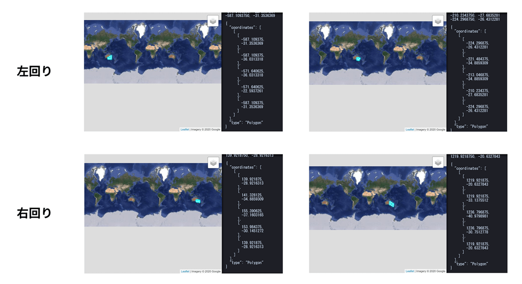
ただし、どちらに移動するのかを考えるのも手間です。そこで、今回は条件分岐を追加してみました。
#左回りもしくは右回りに対応
for i in range(len(AREA)):
    if AREA[i][0] >= 0:
        AREA[i][0] = AREA[i][0]%360
    else:
        AREA[i][0] = -(abs(AREA[i][0])%360) + 360
あとは前回同様関心領域のポリゴンを作成します。
from geojson import Polygon
m=Polygon([AREA])

#確認するエリア名に変更してください
object_name = 'Balmoral'

import json
with open(str(object_name) +'.geojson', 'w') as f:
    json.dump(m, f)

footprint_geojson = geojson_to_wkt(read_geojson(str(object_name) +'.geojson'))
過去記事に従ってSentinel APIを登録の上、下記に情報を埋めてください。
user = '自身のアカウント情報を記載してください'
password = '自身のアカウントのパスワードを記載してください'

api = SentinelAPI(user, password, 'https://scihub.copernicus.eu/dhus')
意図したエリアのポリゴンを作成できているか確認します。
m = folium.Map([(AREA[0][1]+AREA[len(AREA)-1][1])/2,(AREA[0][0]+AREA[len(AREA)-1][0])/2], zoom_start=10)

folium.GeoJson(str(object_name) +'.geojson').add_to(m)
m
続いて、画像に埋め込むフォントを指定します。
!xz -dc mplus-TESTFLIGHT-*.tar.xz | tar xf -
cwd = os.getcwd()
suffix = '.ttf'
base_filename = 'mplus-1c-bold'
fontfile = os.path.join(cwd,'mplus-TESTFLIGHT-063a',base_filename + suffix)
では、画像を取得する準備をしていきましょう。
def Sentinel2_get_init(i):
    products = api.query(footprint_geojson,
                     date = (Begin_date, End_date1), #画像取得月の画像取得
                     platformname = 'Sentinel-2',
                     processinglevel = 'Level-2A', #Leve-1C
                     cloudcoverpercentage = (0,100)) #被雲率(0%〜50%)

    products_gdf = api.to_geodataframe(products)

    #画像取得月の被雲率の小さい画像からソートする.
    products_gdf_sorted = products_gdf.sort_values(['cloudcoverpercentage'], ascending=[True])
    title = products_gdf_sorted.iloc[i]["title"]
    print(str(title))

    uuid = products_gdf_sorted.iloc[i]["uuid"]
    product_title = products_gdf_sorted.iloc[i]["title"]

    #画像の観測日を確認.
    date = products_gdf_sorted.iloc[i]["ingestiondate"].strftime('%Y-%m-%d')
    print(date)

    #Sentinel-2 data download
    api.download(uuid)
    file_name = str(product_title) +'.zip'


    #ダウロードファイルの解凍.
    with zipfile.ZipFile(file_name) as zf:
        zf.extractall()

    #フォルダの画像ファイルのアドレスを取得.
    path = str(product_title) + '.SAFE/GRANULE'
    files = os.listdir(path)
    pathA = str(product_title) + '.SAFE/GRANULE/' + str(files[0])
    files2 = os.listdir(pathA)
    pathB = str(product_title) + '.SAFE/GRANULE/' + str(files[0]) +'/' + str(files2[1]) +'/R10m'
    files3 = os.listdir(pathB)


    path_b2 = str(product_title) + '.SAFE/GRANULE/' + str(files[0]) +'/' + str(files2[1]) +'/R10m/' +str(files3[0][0:23] +'B02_10m.jp2')
    path_b3 = str(product_title) + '.SAFE/GRANULE/' + str(files[0]) +'/' + str(files2[1]) +'/R10m/' +str(files3[0][0:23] +'B03_10m.jp2')
    path_b4 = str(product_title) + '.SAFE/GRANULE/' + str(files[0]) +'/' + str(files2[1]) +'/R10m/' +str(files3[0][0:23] +'B04_10m.jp2')

    # Band4,3,2をR,G,Bとして開く.
    b4 = rio.open(path_b4)
    b3 = rio.open(path_b3)
    b2 = rio.open(path_b2)

    #RGBカラー合成(GeoTiffファイルの出力)
    with rio.open(str(object_name) +'.tiff','w',driver='Gtiff', width=b4.width, height=b4.height,
              count=3,crs=b4.crs,transform=b4.transform, dtype=b4.dtypes[0]) as rgb:
        rgb.write(b4.read(1),1)
        rgb.write(b3.read(1),2)
        rgb.write(b2.read(1),3)
        rgb.close()

    #ポリゴン情報の取得.
    nReserve_geo = gpd.read_file(str(object_name) +'.geojson')

    #取得画像のEPSGを取得
    epsg = b4.crs

    nReserve_proj = nReserve_geo.to_crs({'init': str(epsg)})

    #マスクTiffファイルの一時置き場
    os.makedirs('./Image_tiff', exist_ok=True)

    #カラー合成画像より関心域を抽出.
    with rio.open(str(object_name) +'.tiff') as src:
        out_image, out_transform = rio.mask.mask(src, nReserve_proj.geometry,crop=True)
        out_meta = src.meta.copy()
        out_meta.update({"driver": "GTiff",
                     "height": out_image.shape[1],
                     "width": out_image.shape[2],
                     "transform": out_transform})

    with rasterio.open('./Image_tiff/' +'Masked_' +str(object_name) +'.tif', "w", **out_meta) as dest:
        dest.write(out_image)

    #抽出画像のjpeg処理.
    scale = '-scale 0 250 0 30'
    options_list = [
        '-ot Byte',
        '-of JPEG',
        scale
    ]

    options_string = " ".join(options_list)

    #ディレクトリの作成
    os.makedirs('./Image_jpeg_'+str(object_name), exist_ok=True)

    #jpeg画像の保存.
    gdal.Translate('./Image_jpeg_'+str(object_name) +'/' + str(Begin_date) + 'Masked_' +str(object_name) +'.jpg',
                   './Image_tiff/Masked_' +str(object_name) +'.tif',
                   options=options_string)

    #画像への撮像日を記載
    img = Image.open('./Image_jpeg_'+str(object_name) +'/' + str(Begin_date) + 'Masked_' +str(object_name) +'.jpg')

    #print(img.size)
    #print(img.size[0])
    x = img.size[0]/100 #日付の記載位置の設定
    y = img.size[1]/100 #日付の記載位置の設定
    fs = img.size[0]/50 #日付のフォントサイズの設定
    fs1 = int(fs)
    #print(fs1)
    #print(type(fs1))
    obj_draw = ImageDraw.Draw(img)
    obj_font = ImageFont.truetype(fontfile, fs1)
    obj_draw.text((x, y), str(date), fill=(255, 255, 255), font=obj_font)
    obj_draw.text((img.size[0]/2, img.size[1]-y - img.size[1]/20 ), 'produced from ESA remote sensing data', fill=(255, 255, 255), font=obj_font)


    img.save('./Image_jpeg_'+str(object_name) +'/' + str(Begin_date) + 'Masked_' +str(object_name) +'.jpg')

    #大容量のダウンロードファイル,および解凍フォルダの削除
    shutil.rmtree( str(product_title) + '.SAFE')
    os.remove(str(product_title) +'.zip')

    return

def Sentinel2_get():
    products = api.query(footprint_geojson,
                     date = (Begin_date, End_date), #取得希望期間の入力
                     platformname = 'Sentinel-2',
                     processinglevel = 'Level-2A', #Leve-1C
                     cloudcoverpercentage = (0,100)) #被雲率(0%〜50%)

    products_gdf = api.to_geodataframe(products)
    products_gdf_sorted = products_gdf.sort_values(['cloudcoverpercentage'], ascending=[True])

    #同一シーンの画像を取得するため,placenumberを固定する.
    products_gdf_sorted = products_gdf_sorted[products_gdf_sorted["title"].str.contains(placenumber)]
    title = products_gdf_sorted.iloc[0]["title"]
    print(str(title))

    uuid = products_gdf_sorted.iloc[0]["uuid"]
    product_title = products_gdf_sorted.iloc[0]["title"]


    date = products_gdf_sorted.iloc[0]["ingestiondate"].strftime('%Y-%m-%d')
    print(date)

    api.download(uuid)
    file_name = str(product_title) +'.zip'

    with zipfile.ZipFile(file_name) as zf:
        zf.extractall()

    path = str(product_title) + '.SAFE/GRANULE'
    files = os.listdir(path)
    pathA = str(product_title) + '.SAFE/GRANULE/' + str(files[0])
    files2 = os.listdir(pathA)
    pathB = str(product_title) + '.SAFE/GRANULE/' + str(files[0]) +'/' + str(files2[1]) +'/R10m'
    files3 = os.listdir(pathB)


    path_b2 = str(product_title) + '.SAFE/GRANULE/' + str(files[0]) +'/' + str(files2[1]) +'/R10m/' +str(files3[0][0:23] +'B02_10m.jp2')
    path_b3 = str(product_title) + '.SAFE/GRANULE/' + str(files[0]) +'/' + str(files2[1]) +'/R10m/' +str(files3[0][0:23] +'B03_10m.jp2')
    path_b4 = str(product_title) + '.SAFE/GRANULE/' + str(files[0]) +'/' + str(files2[1]) +'/R10m/' +str(files3[0][0:23] +'B04_10m.jp2')

    b4 = rio.open(path_b4)
    b3 = rio.open(path_b3)
    b2 = rio.open(path_b2)

    with rio.open(str(object_name) +'.tiff','w',driver='Gtiff', width=b4.width, height=b4.height,
              count=3,crs=b4.crs,transform=b4.transform, dtype=b4.dtypes[0]) as rgb:
        rgb.write(b4.read(1),1)
        rgb.write(b3.read(1),2)
        rgb.write(b2.read(1),3)
        rgb.close()

    os.makedirs('./Image_tiff', exist_ok=True)

    nReserve_geo = gpd.read_file(str(object_name) +'.geojson')
    epsg = b4.crs

    nReserve_proj = nReserve_geo.to_crs({'init': str(epsg)})

    with rio.open(str(object_name) +'.tiff') as src:
        out_image, out_transform = rio.mask.mask(src, nReserve_proj.geometry,crop=True)
        out_meta = src.meta.copy()
        out_meta.update({"driver": "GTiff",
                     "height": out_image.shape[1],
                     "width": out_image.shape[2],
                     "transform": out_transform})

    with rasterio.open('./Image_tiff/' +'Masked_' +str(object_name) +'.tif', "w", **out_meta) as dest:
        dest.write(out_image)

    from osgeo import gdal

    scale = '-scale 0 250 0 30'
    options_list = [
        '-ot Byte',
        '-of JPEG',
        scale
    ]
    options_string = " ".join(options_list)

    os.makedirs('./Image_jpeg_'+str(object_name), exist_ok=True)

    gdal.Translate('./Image_jpeg_'+str(object_name) +'/' + str(Begin_date) + 'Masked_' +str(object_name) +'.jpg',
                   './Image_tiff/Masked_' +str(object_name) +'.tif',
                   options=options_string)

    #画像への撮像日の記載
    img = Image.open('./Image_jpeg_'+str(object_name) +'/' + str(Begin_date) + 'Masked_' +str(object_name) +'.jpg')

    #print(img.size)
    #print(img.size[0])
    x = img.size[0]/100 #日付の記載位置の設定
    y = img.size[1]/100 #日付の記載位置の設定
    fs = img.size[0]/50 #日付のフォントサイズの設定
    fs1 = int(fs)
    #print(fs1)
    #print(type(fs1))
    obj_draw = ImageDraw.Draw(img)
    obj_font = ImageFont.truetype(fontfile, fs1)
    obj_draw.text((x, y), str(date), fill=(255, 255, 255), font=obj_font)
    obj_draw.text((img.size[0]/2, img.size[1]-y - img.size[1]/20 ), 'produced from ESA remote sensing data', fill=(255, 255, 255), font=obj_font)
    img.save('./Image_jpeg_'+str(object_name) +'/' + str(Begin_date) + 'Masked_' +str(object_name) +'.jpg')

    shutil.rmtree( str(product_title) + '.SAFE')
    os.remove(str(product_title) +'.zip')

    return
画像を取得する期間を指定します。
#L2Aデータ取得のため,2019年1月以降を開始日とすること.
Begin_date = '20190101'
End_date1 = Begin_date[:6] +'28'#月の終わりを28としているのは,2月を考慮して.
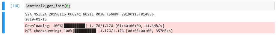
開始月の画像を確認します。被雲率の小さい画像から確認するため、引数は0とします。
Sentinel2_get_init(0)実行すると例えば下記のように表示されます。
S2A_MSIL2A_20190115T000241_N0211_R030_T56HKH_20190115T014856における”T56HKH”の部分をコピーしましょう。
2. 関心領域のGIFアニメーションを作成する
では、上記情報を元にGIFアニメーションを作成していきましょう。各月で最も雲が少ない画像を選定のうえ、GIFアニメーションにします。
placenumber = '_T56HKH_' #上記で取得したplacenumberを貼り付けます

#L2Aデータ取得の場合は、2019年1月以降を開始日とすること
Begin_date = '20190101'
End_date = '20200131'

#年をまたぐ画像を取得する場合のため、以下のコードにて月数をカウントする
d_year = int(End_date[2:4]) - int(Begin_date[2:4])
d_year = d_year*12 + int(End_date[4:6]) - int(Begin_date[4:6])
各月の衛星画像の取得し、関心領域のjpeg画像を作成します。
for i in range(d_year):
    if i < 1:
        m = int(Begin_date[4:6])
    else:
        m = int(Begin_date[4:6]) +1

    if m <10:
        Begin_date = Begin_date[:4] +'0'+ str(m) + Begin_date[6:]
    elif m <13:
        Begin_date = Begin_date[:4] + str(m) + Begin_date[6:]
    else:
        y = int(Begin_date[2:4]) +1
        Begin_date = Begin_date[:2] + str(y) + '01' + Begin_date[6:]
    End_date = Begin_date[:6] +'28'

    Sentinel2_get()
作成したjpeg画像を、古い観測画像よりGIFアニメーションにします。
images =[]

files = sorted(glob.glob('./Image_jpeg_'+str(object_name) +'/*.jpg'))
images = list(map(lambda file: Image.open(file), files))

images[0].save('./Image_jpeg_'+str(object_name) +'/' + str(object_name) + '.gif', save_all=True, append_images=images[1:], duration=1000, loop=0)
今回指定した領域の場合には、下記のようなアニメーションを取得できます。
下記はオーストラリアで林野火災の被害が大きく出ていたバルモラル周辺の画像を取得しました。火災により、森林面積が減っている様子を感じ取れるかと思います。
ただし、これが林野火災によるものなのか、季節変化(オーストラリアは南半球なので季節が日本と逆)によるものなのか、を結論付けるには、可視化するデータを変えることや、データを取得する頻度を上げる、などもう少し情報が必要となります。観測頻度を上げる方法については、また別の記事でご紹介予定です。
~宙畑コラム~
取得した4月の画像を見たとき、何やら不思議な点に気づかれた方もいるかもしれません。
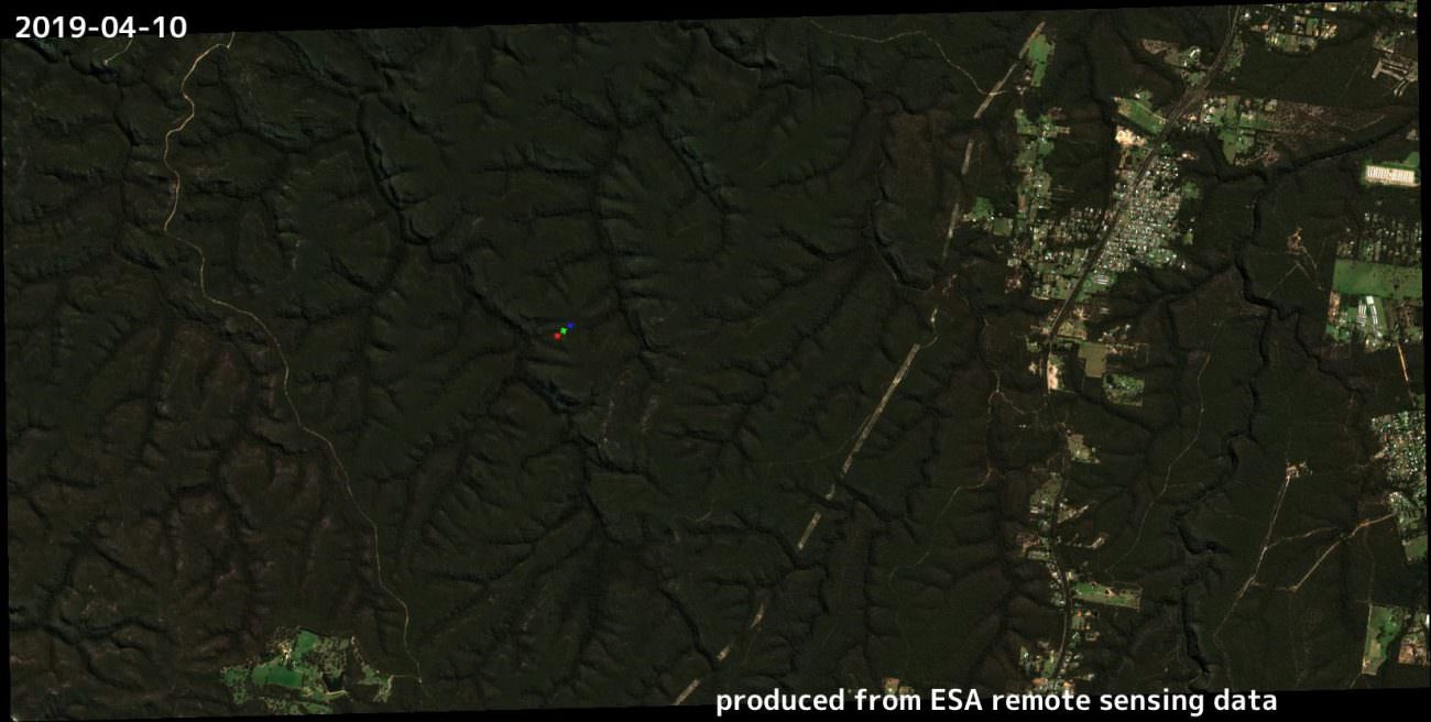
それは、画像中央左にある、RGBの3つの点。拡大すると航空機の形であることが分かるかと思います。
これは、衛星の不具合ではなく、衛星に搭載しているカメラの性質によるものです。
私たちが普段利用しているカメラではこのような現象が起きないのに、なぜ衛星に搭載しているカメラでこのような現象が生じるのか?
答えは、衛星に搭載されているカメラはバンドごとにスキャンしながら撮影するからです。
つまり、バンドRとGとBなどを別々のタイミング(とは言えかなりの速さでスキャンしているのですが)で撮影しているため、航空機のように高速で移動している対象を撮影する場合には、このように分離して見えるのです。
※興味のある方はRGBの距離と航空機の平均的な巡航速度から、撮影する速さを求めてみるのも面白いですよ
—-
3. バンドを変えて画像を取得する
利用する画像を指定する際に、2章では下記のように記載していました。該当するGRANULEのフォルダにアクセスしてみた方の中には、他のバンドの画像も格納されていることに気が付いた方もいらっしゃるかもしれません。
path = str(product_title) + '.SAFE/GRANULE'
    files = os.listdir(path)
    pathA = str(product_title) + '.SAFE/GRANULE/' + str(files[0])
    files2 = os.listdir(pathA)
    pathB = str(product_title) + '.SAFE/GRANULE/' + str(files[0]) +'/' + str(files2[1]) +'/R10m'
    files3 = os.listdir(pathB)


    path_b2 = str(product_title) + '.SAFE/GRANULE/' + str(files[0]) +'/' + str(files2[1]) +'/R10m/' +str(files3[0][0:23] +'B02_10m.jp2')
    path_b3 = str(product_title) + '.SAFE/GRANULE/' + str(files[0]) +'/' + str(files2[1]) +'/R10m/' +str(files3[0][0:23] +'B03_10m.jp2')
    path_b4 = str(product_title) + '.SAFE/GRANULE/' + str(files[0]) +'/' + str(files2[1]) +'/R10m/' +str(files3[0][0:23] +'B04_10m.jp2')
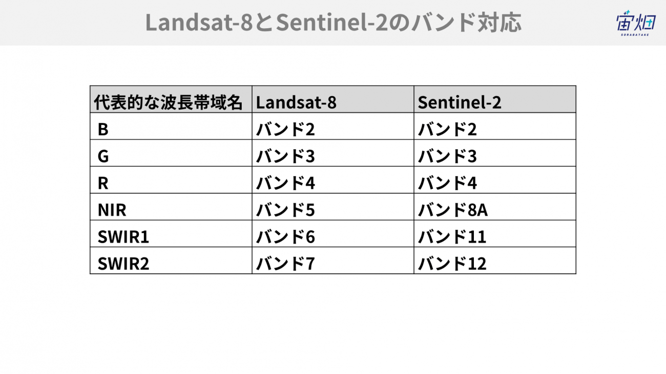
この中で、熱源検知に役立つ組み合わせとして、短波長赤外域(SWIR)を利用した組み合わせが良い、と宙畑の記事で紹介されています。
先の記事ではLandsat-8を利用しているため、組み合わせはRが7、Gが6、Bが5でした。今回利用しているSentinel-2の場合は、Rが12、Gが11、Bが8Aに該当します。この割り当てに下記のように変更することで、熱源(熱を持っている範囲)を目立たせた画像を取得できます。
Sentinel2_get_init(i)とSentinel2_get()それぞれの関数の中に該当箇所があるのでそれぞれ変更します。
path = str(product_title) + '.SAFE/GRANULE'
    files = os.listdir(path)
    pathA = str(product_title) + '.SAFE/GRANULE/' + str(files[0])
    files2 = os.listdir(pathA)
    pathB = str(product_title) + '.SAFE/GRANULE/' + str(files[0]) +'/' + str(files2[1]) +'/R20m'
    files3 = os.listdir(pathB)


    path_b2 = str(product_title) + '.SAFE/GRANULE/' + str(files[0]) +'/' + str(files2[1]) +'/R20m/' +str(files3[0][0:23] +'B8A_20m.jp2')
    path_b3 = str(product_title) + '.SAFE/GRANULE/' + str(files[0]) +'/' + str(files2[1]) +'/R20m/' +str(files3[0][0:23] +'B11_20m.jp2')
    path_b4 = str(product_title) + '.SAFE/GRANULE/' + str(files[0]) +'/' + str(files2[1]) +'/R20m/' +str(files3[0][0:23] +'B12_20m.jp2')
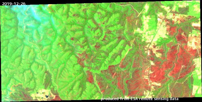
なお、組み合わせをRが12、Gが8A、Bが4のようにすると、下記のような画像を取得できます。直観的にはこちらの方が発災の様子を捉えやすいですね。
バンド12(SWIR)は輻射と反射が混ざったバンドなのに対して、バンド8A(NIR)やバンド4(R)は反射だけを捉えているので、SWIRを赤に割り当てた時に、輻射(要は熱を発しているかどうか)の影響が見やすくなるのです。
分解能が10mから20mになったことから、いずれの画像からも4月に見えていた航空機が見えなくなっています。その代わり、2章のRGBで描画していたときと異なり、12月に生じた林野火災の影響でバルモラルの町周辺が真っ赤に見えています。赤いところは熱を発しているところ、つまりは広範囲にわたり火災が起きていたことが分かります。
4. まとめ
以上、指定した範囲における各月で最も被雲率の低い画像を選択し、アニメーションを作成する方法でした。詳細な解説はQiitaにも公開していますので、よろしければ合わせてご覧ください。
今回は被害状況が深刻なオーストラリアを対象に画像を取得しました。字面で見ているだけよりも、データとして確認した方が実際の被災状況を適切に把握できることが多くあります。実際に12月の画像から、被災範囲の広さに驚かれた方も多くいたのではないでしょうか?
広範囲に観測している衛星データの特徴を利用することで、ニュースで報道されていないけれども、実は被災状況がより甚大な地域を発見することもできるかもしれません。また、次に林野火災が発生しそうな地域を予測することもできるかもしれません。
そうすると、より適切に支援することもできるかもしれませんよね。無料の衛星画像からも多くの情報を得ることができます。まずは状態を正しく知ることが重要です。
今回のような使い方でない場合には、例えば田んぼの育成状況を把握する上で利用することも可能です。
青森の田んぼの時間変化を確認すると下記のようになります。青々と茂った田んぼが秋ごろの収穫時期に向けて黄金色となり、そして土壌が見えるように変化していることが分かるかと思います。
これ以外にも時系列変化を確認することで分かることが様々にあります。皆さまも関心のある地域の画像を取得し、その変化を見てみてください。
関連記事
オーストラリア 森林火災の衛星画像のタイムラプスを作ってみた.