【コード付き】Sentinel-2から指定した範囲の連続した衛星画像を取得する
林野火災による被害が大きいオーストラリアを対象に、林野火災が目立つようにブレンドした衛星画像を指定期間分取得してタイムラプスを作成し、その被害状況を可視化する方法をご紹介します。
記事作成時から、Tellusからデータを検索・取得するAPIが変更になっております。該当箇所のコードについては、以下のリンクをご参照ください。
https://www.tellusxdp.com/ja/howtouse/access/traveler_api_20220310_
firstpart.html
2022年8月31日以降、Tellus OSでのデータの閲覧方法など使い方が一部変更になっております。新しいTellus OSの基本操作は以下のリンクをご参照ください。
https://www.tellusxdp.com/ja/howtouse/tellus_os/start_tellus_os.html
過去の記事では、指定した期間の各月で最も被雲率の低い衛星画像をAPIで取得し、タイムラプスを作成する方法をご紹介しました。
しかしながら、月に1枚の画像で作成したタイムラプスでは、知りたい情報を知る上で不十分な場合もあります。
長期的に森林の保全状況を見たい場合はダウンロードするデータ量などの観点からも月に1度程度の時間分解能の方が良いですが、被災状況などの短期的な変化を確認したい場合はなるべく期間を空けずに見られる方が望ましいですよね。
そこで、本記事では同じく豪州の林野火災を対象に、5日ごとの衛星画像を取得し、タイムラプスを作成する方法をご紹介します。
1. 対象エリアを選定
流れとしては過去記事と同様です。今回は前半部分の説明は省略します。気になる方は過去記事をご覧ください。
import os
import numpy as np

from sentinelsat import SentinelAPI, read_geojson, geojson_to_wkt
import geopandas as gpd
import pandas as pd
import numpy as np
import matplotlib.pyplot as plt

from shapely.geometry import MultiPolygon, Polygon
import rasterio as rio
from rasterio.plot import show
import rasterio.mask
import fiona
import folium

#関心領域のポリゴン情報の取得
from IPython.display import HTML
HTML(r' width="960" height="480" src="https://www.keene.edu/campus/maps/tool/" frameborder="0">')
#実行する際には上記r’の次に、<iframeの文字列(<は半角)をコピー・挿入して実行してください
#上記にて取得した地理情報をコピペ.
AREA =  [
      [
        -210.4512048,
        -35.2522692
      ],
      [
        -210.4512048,
        -35.2477833
      ],
      [
        -210.4525244,
        -35.8537092
      ],
      [
        -209.5915246,
        -35.8444562
      ],
      [
        -209.5799482,
        -35.2564395
      ],
      [
        -210.4512048,
        -35.2522692
      ]
    ]


#左回りもしくは右回りに対応
for i in range(len(AREA)):
    if AREA[i][0] >= 0:
        AREA[i][0] = AREA[i][0]%360
    else:
        AREA[i][0] = -(abs(AREA[i][0])%360) + 360

#関心域の地理情報ポリゴンの作成
from geojson import Polygon
m=Polygon([AREA])

#確認するエリア名に変更してください
object_name = 'Australia_wildfire'

import json
with open(str(object_name) +'.geojson', 'w') as f:
    json.dump(m, f)

footprint_geojson = geojson_to_wkt(read_geojson(str(object_name) +'.geojson'))

#意図したエリアのポリゴンを作成できているか確認する
m = folium.Map([(AREA[0][1]+AREA[len(AREA)-1][1])/2,(AREA[0][0]+AREA[len(AREA)-1][0])/2], zoom_start=10)

folium.GeoJson(str(object_name) +'.geojson').add_to(m)
m

#利用するフォントを設定する
!xz -dc mplus-TESTFLIGHT-*.tar.xz | tar xf -
cwd = os.getcwd()
suffix = '.ttf'
base_filename = 'mplus-1c-bold'
fontfile = os.path.join(cwd,'mplus-TESTFLIGHT-063a',base_filename + suffix)
2. Sentinel-2の衛星画像取得,およびGIFアニメーション作成の関数の準備
user = '自身のアカウント情報を記載してください'
password = '自身のアカウントのパスワードを記載してください'

api = SentinelAPI(user, password, 'https://scihub.copernicus.eu/dhus')
下記関数については、基本的に過去の記事と同様の構成ですが、細かく以下の点を変更しています。
まず、一般的な人工衛星から取得した観測画像(True Color)とは異なり、林野火災を見やすくするために、Sentinel-2の赤外波長の画像(B12, B11, B8A)を使用します。
また、林野火災が目立つようにscaleの中の最大値も小さく変更しています。scaleの中の値は下記のように定義されています。
scale [src_min,src_max,dst_min,dst_max]
詳細はこちらをご確認ください。
他には、せっかくダウンロードした後に思っていたのと違う場所のデータを取得していたら嫌ですよね。ということで、下記のように取得したデータのサムネイルを表示できるように変更を加えています。
    #サムネイルを表示
    img_arr = np.asarray(img) #画像をarrayに変換
    print(img_arr.shape)
    plt.imshow(img_arr)
    plt.show()


def Sentinel2_get_init(i):
    products = api.query(footprint_geojson,
                     date = (Begin_date, End_date), #画像取得月の画像取得
                     platformname = 'Sentinel-2',
                     processinglevel = 'Level-2A', #Leve-1C
                     cloudcoverpercentage = (0,50)) #被雲率

    products_gdf = api.to_geodataframe(products)

    #画像取得月の被雲率の小さい画像からソートする.
    products_gdf_sorted = products_gdf.sort_values(['cloudcoverpercentage'], ascending=[True])
    title = products_gdf_sorted.iloc[i]["title"]
    print(str(title))

    uuid = products_gdf_sorted.iloc[i]["uuid"]
    product_title = products_gdf_sorted.iloc[i]["title"]

    #画像の観測日を確認.
    date = products_gdf_sorted.iloc[i]["ingestiondate"].strftime('%Y-%m-%d')
    print(date)

    #Sentinel-2 data download
    api.download(uuid)
    file_name = str(product_title) +'.zip'


    #ダウロードファイルの解凍.
    with zipfile.ZipFile(file_name) as zf:
        zf.extractall()

    #フォルダの画像ファイルのアドレスを取得.
    path = str(product_title) + '.SAFE/GRANULE'
    files = os.listdir(path)
    pathA = str(product_title) + '.SAFE/GRANULE/' + str(files[0])
    files2 = os.listdir(pathA)
    pathB = str(product_title) + '.SAFE/GRANULE/' + str(files[0]) +'/' + str(files2[1]) +'/R20m'
    files3 = os.listdir(pathB)


    path_b12 = str(product_title) + '.SAFE/GRANULE/' + str(files[0]) +'/' + str(files2[1]) +'/R20m/' +str(files3[0][0:23] +'B12_20m.jp2')
    path_b11 = str(product_title) + '.SAFE/GRANULE/' + str(files[0]) +'/' + str(files2[1]) +'/R20m/' +str(files3[0][0:23] +'B11_20m.jp2')
    path_b8 = str(product_title) + '.SAFE/GRANULE/' + str(files[0]) +'/' + str(files2[1]) +'/R20m/' +str(files3[0][0:23] +'B8A_20m.jp2')

    # Band4,3,2をR,G,Bとして開く.
    b8 = rio.open(path_b8)
    b12 = rio.open(path_b12)
    b11 = rio.open(path_b11)

    #RGBカラー合成(GeoTiffファイルの出力)
    with rio.open(str(object_name) +'.tiff','w',driver='Gtiff', width=b12.width, height=b12.height,
              count=3,crs=b12.crs,transform=b12.transform, dtype=b12.dtypes[0]) as rgb:
        rgb.write(b12.read(1),1)
        rgb.write(b11.read(1),2)
        rgb.write(b8.read(1),3)
        rgb.close()

    #ポリゴン情報の取得.
    nReserve_geo = gpd.read_file(str(object_name) +'.geojson')

    #取得画像のEPSGを取得
    epsg = b12.crs

    nReserve_proj = nReserve_geo.to_crs({'init': str(epsg)})

    #マスクTiffファイルの一時置き場
    os.makedirs('./Image_tiff', exist_ok=True)

    #カラー合成画像より関心域を抽出.
    with rio.open(str(object_name) +'.tiff') as src:
        out_image, out_transform = rio.mask.mask(src, nReserve_proj.geometry,crop=True)
        out_meta = src.meta.copy()
        out_meta.update({"driver": "GTiff",
                     "height": out_image.shape[1],
                     "width": out_image.shape[2],
                     "transform": out_transform})

    with rasterio.open('./Image_tiff/' +'Masked_' +str(object_name) +'.tif', "w", **out_meta) as dest:
        dest.write(out_image)

    #抽出画像のjpeg処理.
    scale = '-scale 0 255 0 15'
    options_list = [
        '-ot Byte',
        '-of JPEG',
        scale
    ]

    options_string = " ".join(options_list)

    #ディレクトリの作成
    os.makedirs('./Image_jpeg_'+str(object_name), exist_ok=True)

    #jpeg画像の保存.
    gdal.Translate('./Image_jpeg_'+str(object_name) +'/' + str(date) + 'Masked_' +str(object_name) +'.jpg',
                   './Image_tiff/Masked_' +str(object_name) +'.tif',
                   options=options_string)

    #画像への撮像日を記載
    img = Image.open('./Image_jpeg_'+str(object_name) +'/' + str(date) + 'Masked_' +str(object_name) +'.jpg')

    #サムネイルを表示
    img_arr = np.asarray(img) #画像をarrayに変換
    print(img_arr.shape)
    plt.imshow(img_arr)
    plt.show()

    x = img.size[0]/100 #日付の記載位置の設定
    y = img.size[1]/100 #日付の記載位置の設定
    fs = img.size[0]/50 #日付のフォントサイズの設定
    fs1 = int(fs)
    obj_draw = ImageDraw.Draw(img)
    #obj_font = ImageFont.truetype("./font/mplus-1c-bold.ttf", fs1)
    obj_font = ImageFont.truetype(fontfile, fs1)
    obj_draw.text((x, y), str(date), fill=(255, 255, 255), font=obj_font)
    obj_draw.text((img.size[0]/2, img.size[1]-y - img.size[1]/20 ), 'produced from ESA remote sensing data', fill=(255, 255, 255), font=obj_font)


    img.save('./Image_jpeg_'+str(object_name) +'/' + str(date) + 'Masked_' +str(object_name) +'.jpg')


    #Copernicus hubからのダウンロードファイル,および解凍フォルダの削除
    shutil.rmtree( str(product_title) + '.SAFE')
    os.remove(str(product_title) +'.zip')

    return

def Sentinel2_get():
    products = api.query(footprint_geojson,
                     date = (begin, end), #取得希望期間の入力
                     platformname = 'Sentinel-2',
                     processinglevel = 'Level-2A', #Leve-1C
                     cloudcoverpercentage = (0,100)) #被雲率

    products_gdf = api.to_geodataframe(products)
    products_gdf_sorted = products_gdf.sort_values(['cloudcoverpercentage'], ascending=[True])

    #同一シーンの画像を取得するため,placenumberを固定する.
    products_gdf_sorted = products_gdf_sorted[products_gdf_sorted["title"].str.contains(placenumber)]
    title = products_gdf_sorted.iloc[0]["title"]
    print(str(title))

    uuid = products_gdf_sorted.iloc[0]["uuid"]
    product_title = products_gdf_sorted.iloc[0]["title"]


    date = products_gdf_sorted.iloc[0]["ingestiondate"].strftime('%Y%m%d')
    date1 = products_gdf_sorted.iloc[0]["ingestiondate"].strftime('%Y-%m-%d')
    print(date)

    api.download(uuid)
    file_name = str(product_title) +'.zip'

    with zipfile.ZipFile(file_name) as zf:
        zf.extractall()

    path = str(product_title) + '.SAFE/GRANULE'
    files = os.listdir(path)
    pathA = str(product_title) + '.SAFE/GRANULE/' + str(files[0])
    files2 = os.listdir(pathA)
    pathB = str(product_title) + '.SAFE/GRANULE/' + str(files[0]) +'/' + str(files2[1]) +'/R20m'
    files3 = os.listdir(pathB)


    path_b12 = str(product_title) + '.SAFE/GRANULE/' + str(files[0]) +'/' + str(files2[1]) +'/R20m/' +str(files3[0][0:23] +'B12_20m.jp2')
    path_b11 = str(product_title) + '.SAFE/GRANULE/' + str(files[0]) +'/' + str(files2[1]) +'/R20m/' +str(files3[0][0:23] +'B11_20m.jp2')
    path_b8 = str(product_title) + '.SAFE/GRANULE/' + str(files[0]) +'/' + str(files2[1]) +'/R20m/' +str(files3[0][0:23] +'B8A_20m.jp2')

    # Band4,3,2をR,G,Bとして開く.
    b8 = rio.open(path_b8)
    b12 = rio.open(path_b12)
    b11 = rio.open(path_b11)

    #RGBカラー合成(GeoTiffファイルの出力)
    with rio.open(str(object_name) +'.tiff','w',driver='Gtiff', width=b12.width, height=b12.height,
              count=3,crs=b12.crs,transform=b12.transform, dtype=b12.dtypes[0]) as rgb:
        rgb.write(b12.read(1),1)
        rgb.write(b11.read(1),2)
        rgb.write(b8.read(1),3)
        rgb.close()

    os.makedirs('./Image_tiff', exist_ok=True)

    nReserve_geo = gpd.read_file(str(object_name) +'.geojson')
    epsg = b12.crs

    nReserve_proj = nReserve_geo.to_crs({'init': str(epsg)})

    with rio.open(str(object_name) +'.tiff') as src:
        out_image, out_transform = rio.mask.mask(src, nReserve_proj.geometry,crop=True)
        out_meta = src.meta.copy()
        out_meta.update({"driver": "GTiff",
                     "height": out_image.shape[1],
                     "width": out_image.shape[2],
                     "transform": out_transform})

    with rasterio.open('./Image_tiff/' +'Masked_' +str(object_name) +'.tif', "w", **out_meta) as dest:
        dest.write(out_image)

    from osgeo import gdal

    scale = '-scale 0 255 0 15'
    options_list = [
        '-ot Byte',
        '-of JPEG',
        scale
    ]
    options_string = " ".join(options_list)

    os.makedirs('./Image_jpeg_'+str(object_name), exist_ok=True)

    gdal.Translate('./Image_jpeg_'+str(object_name) +'/' + str(date) + 'Masked_' +str(object_name) +'.jpg',
                   './Image_tiff/Masked_' +str(object_name) +'.tif',
                   options=options_string)

    #画像への撮像日の記載
    img = Image.open('./Image_jpeg_'+str(object_name) +'/' + str(date) + 'Masked_' +str(object_name) +'.jpg')

    #サムネイルを表示
    img = Image.open('./Image_jpeg_'+str(object_name) +'/' + str(date) + 'Masked_' +str(object_name) +'.jpg')
    img_arr = np.asarray(img) #画像をarrayに変換
    print(img_arr.shape)
    plt.imshow(img_arr)
    plt.show()

    x = img.size[0]/100 #日付の記載位置の設定
    y = img.size[1]/100 #日付の記載位置の設定
    fs = img.size[0]/50 #日付のフォントサイズの設定
    fs1 = int(fs)
    obj_draw = ImageDraw.Draw(img)
    obj_font = ImageFont.truetype(fontfile, fs1)
    obj_draw.text((x, y), str(date1), fill=(0, 0, 128), font=obj_font) #Red:(255, 0, 0), Blue:(0,0,255), Navy:(0,0,128),Yellow:(255,255,0), bluegreen:(0,128,128),Perple:(128,0,128)
    obj_draw.text((img.size[0]/2, img.size[1]-y - img.size[1]/20 ), 'produced from ESA remote sensing data', fill=(0, 0, 128), font=obj_font)
    img.save('./Image_jpeg_'+str(object_name) +'/' + str(date) + 'Masked_' +str(object_name) +'.jpg')


    #Copernicus hubからのダウンロードファイル,および解凍フォルダの削除
    shutil.rmtree( str(product_title) + '.SAFE')
    os.remove(str(product_title) +'.zip')

    return
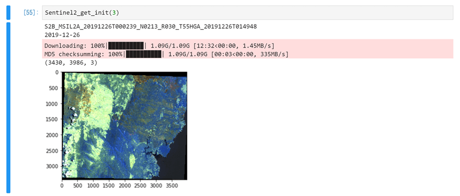
3.取得する衛星画像を確認する
#L2Aデータ取得のため,2019年1月以降を開始日とすること.
Begin_date = '20191215'
End_date = Begin_date[:6] +'28'#1月間の観測画像より,関心域を多く含む画像のタイル番号を取得する.

Sentinel2_get_init(3)
今回の場合は、Sentinel2_get_init(3)とすることで、目的とするエリアの画像を取得できることが分かりました。
そのplacenumberであるT55HGAをコピーの上で次のステップに進みます。
4. 関心領域のGIFアニメーションを作成する
では、上記情報を元にGIFアニメーションを作成していきましょう。前回の記事で2019年末に林野火災が起きていそうなことが分かったことから、12月から1月上旬までのGIFアニメーションにします。Sentinel-2の観測周期は5日が基本なので、5日おきに画像を取得します。
placenumber = '_T55HGA_' #上記で取得したplacenumberを貼り付けます

#L2Aデータ取得の場合は、2019年1月以降を開始日とすること
Begin_date = '20191201'
End_date = '20200110'
m = 5 # 5日間毎の画像を取得する

#開始日と終了日の日差の数を求める.
begin_data_s = datetime.datetime.strptime(Begin_date, '%Y%m%d')
end_data_s = datetime.datetime.strptime(End_date, '%Y%m%d')
d_day = end_data_s - begin_data_s
n =d_day.days//m
過去の記事では各月の衛星画像の取得するように条件分けしていましたが、今回は下記のように条件分けを変更し、関心領域のgif画像を作成します。
for i in range(n):
    if i < 1:
        Begin_date = begin_data_s
        End_date = begin_data_s + datetime.timedelta(days=m)
        begin= Begin_date.strftime('%Y%m%d')
        end = End_date.strftime('%Y%m%d')
    else:
        Begin_date = End_date
        End_date = Begin_date + datetime.timedelta(days=m)
        begin= Begin_date.strftime('%Y%m%d')
        end = End_date.strftime('%Y%m%d')

    Sentinel2_get()

images =[]

files = sorted(glob.glob('./Image_jpeg_'+str(object_name) +'/*.jpg'))
images = list(map(lambda file: Image.open(file), files))

images[0].save('./Image_jpeg_'+str(object_name) +'/' + str(object_name) + '.gif', save_all=True, append_images=images[1:], duration=1000, loop=0)
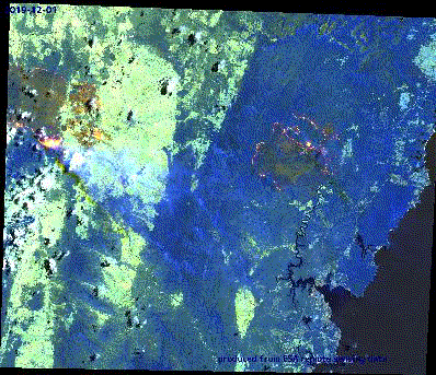
今回指定した領域の場合には、下記のようなアニメーションを取得できます。
大規模な林野火災が発生していることが目に見えて分かります。
さて、読者の中には、なぜSentinel2_get_init(0)ではなく、Sentinel2_get_init(3)としてコードを実行していたのだろうか、と気になった方もいるかと思います。
過去の記事ではSentinel2_get_init(0)と実行して、すんなりと目的とした画像を入手できていました。
しかしながら、今回対象とするエリアでは、Sentinel2_get_init(0)と実行すると、下記のように見たい範囲に対して不十分な画像が取得されてしまうのです。なぜこのようなことが起きるのか、ということについて知りたい方はこちらの記事をご覧ください。
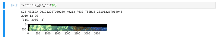
このように、目的に沿った範囲の画像を取得できていないときには、()内の数字を変更しながら、取得したいデータを得られるまで数字を変更しましょう。
ちなみに、上記で得られたplacenumber(T55HGB)を利用した場合には下記のような途切れた画像でgifが作られてしまいます。上記で得られたサムネイル画像と同じ範囲でしか画像を取得できていないことが分かりますね。せっかく時間をかけて出来たgifを見て、あー、、、とならないためにも、placenumberを確認することは重要です。

5.まとめ
以上、指定した範囲における5日おきの画像を取得し、アニメーションを作成する方法でした。詳細な解説はQiitaにも公開していますので、よろしければ合わせてご覧ください。
今回の記事でも被害状況が深刻なオーストラリアを対象に画像を取得しました。過去の記事では熱を発している範囲、つまりは焼けた跡から、燃えていたのであろうことを間接的に把握しただけでした。しかしながら、今回の記事ではデータを取得する頻度を上げたことで、林野火災が実際に発生している瞬間を把握できました。目に見えることで、実際に燃えているのはどの範囲なのか、どの規模でいつ燃えたのか、ということなど、被災状況に対しての理解がさらに深まりますよね。
衛星画像はデータ量が非常に大きいです。そのため、興味のある時間幅をなんとなく決めてデータを取得すると、自身のストレージを圧迫することに繋がります。月に1度程度の頻度で変化を大まかに掴んだ後に、興味が本当にある時期のデータだけ頻度を上げて取得するようにすることで、より効率よくデータを利用できるようになります。適切なデータを取得できれば、現象に対する理解も深めやすくなるという利点もあります。
これ以外にも時系列変化を確認することで分かることが様々にあります。皆さまも関心のある地域の画像を取得し、その変化を見てみてください。
関連記事
https://qiita.com/nigo1973/items/28c873a21fc155a511bf
https://sorabatake.jp/9987/