【コード付き】衛星画像を使って青森県の水田割合の変化を比較する~分析編~
衛星データを使った水田の把握って、実際にやるとしたらどうやるの? 植生の閾値調整、また、面積の計測にチャレンジしてみました。
記事作成時から、Tellusからデータを検索・取得するAPIが変更になっております。該当箇所のコードについては、以下のリンクをご参照ください。
https://www.tellusxdp.com/ja/howtouse/access/traveler_api_20220310_
firstpart.html
2022年8月31日以降、Tellus OSでのデータの閲覧方法など使い方が一部変更になっております。新しいTellus OSの基本操作は以下のリンクをご参照ください。
https://www.tellusxdp.com/ja/howtouse/tellus_os/start_tellus_os.html
衛星データを活用すれば「『青天の霹靂』に聞く!衛星データを用いた広大な稲作地帯の収穫時期予測」のように、美味しいお米作りにも役立てることができます。
ただ、水田の把握ってどうやるの? ということで、実際に衛星データを活用すれば水田の有無が分かるのか、また、面積をどのように測るのかにチャレンジしてみました。
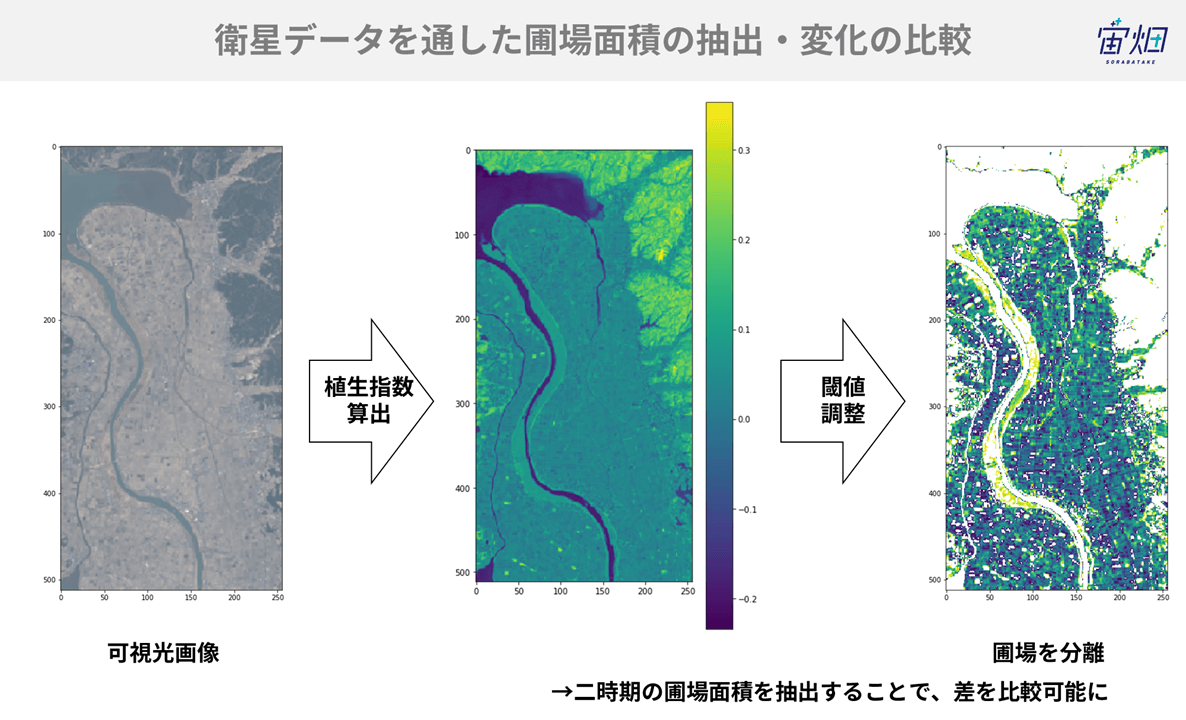
インタビューに伺った青森県の水田を対象に、波長帯を定めた画像データから植生指数(NDVI)を導出し、画像から水田を抽出。また、時系列でデータを眺めたときに、水田の様子はどのように変化しているのかを確認します。
※今回はLandsat-8の衛星データを取得して解析を行います。Landsat-8についての詳しい情報はデータカタログの詳細をご覧ください。
※TellusでJupyter Notebookを使う方法は、「Tellusの開発環境でAPI引っ張ってみた」をご覧ください。
(1)APIを用いてシーン(メタデータ)を取得する
まずは、Landsat-8のシーンを取得するために、APIを利用します。
import os, json, requests, math, glob, re
import numpy as np
from skimage import io
from io import BytesIO
import dateutil.parser
from datetime import datetime
from datetime import timezone
import matplotlib.pyplot as plt
%matplotlib inline

TOKEN = "自分のトークンを入れてください"

def get_landsat_scene(min_lat, min_lon, max_lat, max_lon):
	"""Landsat8のメタデータを取得します"""
	url = "https://gisapi.tellusxdp.com/api/v1/landsat8/scene" \
    	+ "?min_lat={}&min_lon={}&max_lat={}&max_lon={}".format(min_lat, min_lon, max_lat, max_lon)
	headers = {
    	"Authorization": "Bearer " + TOKEN
	}

	r = requests.get(url, headers=headers)
	return r.json()
さっそく弘前周辺のシーンを取得してみましょう。緯度や経度の情報については、Tellus OS上に図形を描き、GeoJSONファイルをダウンロードして調べることができます。
# 弘前周辺
scenes = get_landsat_scene(40.49, 140.502, 40.744, 140.797)
# {\min_lat\:40.49,\min_lon\:140.502,\max_lat\:40.744,\max_lon\:140.797}
print(len(scenes))
# 47
指定した座標の近傍から47個のデータを取得することができました。これらのメタデータは撮影日時の情報を含んでいますので、任意の期間だけのデータを抽出することにします。今回は2014年1月1日から2019年6月1日までを指定します。
def filter_by_date(scenes, start_date=None, end_date=None):
    	"""衛星の撮影時間を基にしてメタデータを抽出する"""
    	if(start_date == None):
        	start_date = datetime(1900,1,1, tzinfo=timezone.utc) # tellusにあるlandsat8のデータは2013年以降から現在まで
    	if(end_date == None):
        	end_date = datetime.now(timezone.utc) # 現在の時間をデフォルトで取得する
    	return [scene for scene in scenes if start_date  dateutil.parser.parse(scene["acquisitionDate"])]

# 2014年1月1日から2019年6月1日まで
landsat_scenes = filter_by_date(scenes, datetime(2014, 1, 1, tzinfo=timezone.utc), datetime(2019, 6, 1, tzinfo=timezone.utc))
print(len(landsat_scenes))
# 43
47個の内、43個が上で指定した期間内に含まれていたようです。念のため、データが範囲内に収まっているかを確かめてみましょう。
ext_date = [re.search(r'\d{2} [A-z]{3} \d{4}',ext_date['acquisitionDate']) for ext_date in landsat_scenes]
period = [i.group() for i in ext_date]
print(period)

たしかに指定していた期間に収まっていますね。では、指定した場所に収まっているかどうか確認するために、これらの全てのサムネイル画像を一括で表示してみます。
def get_tile_images(scenes, r_num, c_num, figsize_x=12, figsize_y=12):
        """サムネイル画像を指定した引数に応じて行列状に表示"""
        thumbs = [imgs['thumbs_url'] for imgs in scenes]
        f, ax_list = plt.subplots(r_num, c_num, figsize=(figsize_x,figsize_y))
        for row_num, ax_row in enumerate(ax_list):
            for col_num, ax in enumerate(ax_row):
                if len(thumbs) < r_num*c_num:
                    len_shortage = r_num*c_num - len(thumbs) # 行列の不足分を算出
                    count = row_num * c_num + col_num
                    if count < len(thumbs):
                        match = re.search(r'\d{2} [A-z]{3} \d{4}',scenes[row_num * c_num + col_num]['acquisitionDate'])
                        D_M_Y = match.group()
                        ax.label_outer() # サブプロットのタイトルと、軸のラベルが被らないようにする
                        ax.imshow(io.imread(thumbs[row_num * c_num + col_num]))
                        ax.set_title(D_M_Y)
                    else:
                        for i in range(len_shortage):
                            blank = np.zeros([100,100,3],dtype=np.uint8)
                            blank.fill(255)
                            ax.label_outer()
                            ax.imshow(blank)
                else:
                    match = re.search(r'\d{2} [A-z]{3} \d{4}',thumbs[row_num * c_num + col_num]['acquisitionDate'])
                    D_M_Y = match.group()
                    ax.label_outer()
                    ax.imshow(io.imread(thumbs[row_num * c_num + col_num]))
                    ax.set_title(D_M_Y)
        return plt.show()

# サムネイル画像を取得
get_tile_images(landsat_scenes,8,6,16,16)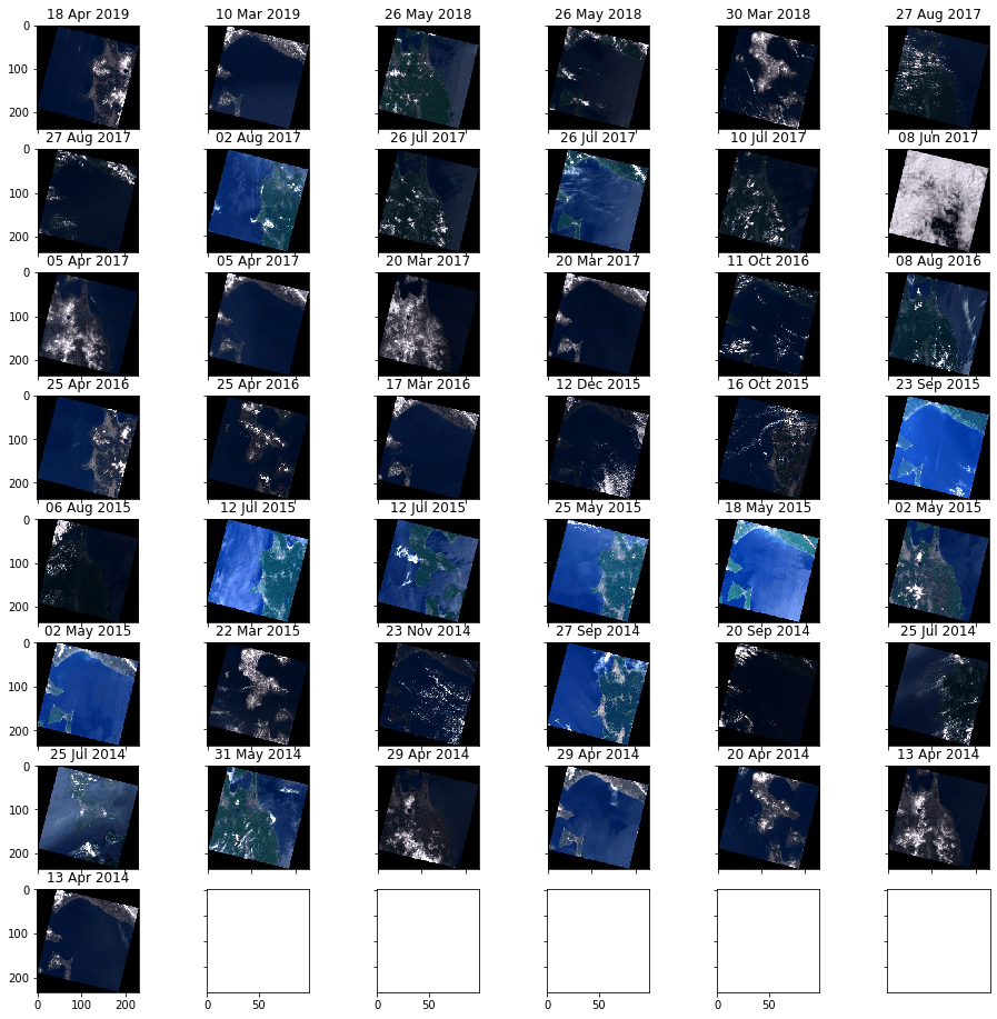
上記のように一覧で表示されました。
今回は年ごとの水田の比較も行いたいので、同じ月のデータで比較ができるように、20 Apr 2014と18 Apr 2019のデータを使います。また、シーンの中から今回は例として青森県北津軽郡中泊町を含んだタイル画像を取得します。
春のデータを指定したのは、対象とした地点に雲や雪がなく、水田も刈り取られたまま草本類も生えていないため、水田を抽出するには適当だと考えられたためです。
# Landsatではタイルデータを取得する場合には、シーンidは指定しない
def get_landsat_image(zoom, xtile, ytile):
	"""取得した画像のタイルを定義し、さらに拡大して表示"""
	url = "https://gisapi.tellusxdp.com/landsat8/{}/{}/{}.png".format(zoom, xtile, ytile)
	headers = {
    	"Authorization": "Bearer " + TOKEN
	}
	r = requests.get(url, headers=headers)
	return io.imread(BytesIO(r.content))


tile01 = get_landsat_image(12, 3645, 1535)
io.imshow(tile01)
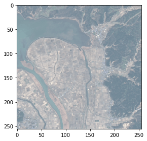
上記のように、中泊町を含んだタイル画像が取得できました。
ここから本題の波長帯を指定した画像抽出に入ります。rgbにどの波長帯を指定するかにより、画像の見映えは変化します。詳しくは「課題に応じて変幻自在? 衛星データをブレンドして見えるモノ・コト」をご覧ください
課題に応じて変幻自在? 衛星データをブレンドして見えるモノ・コト #マンガでわかる衛星データ
def get_landsat_blend(path,row,productId,zoom, xtile, ytile, opacity=1, r=4, g=3, b=2, rdepth=1, gdepth=1, bdepth=1, preset=None):
	url = "https://gisapi.tellusxdp.com/blend/landsat8/{}/{}/{}/{}/{}/{}.png?opacity={}&r={}&g={}&b={}&rdepth={}&gdepth={}&bdepth={}".format\
	(path, row, productId, zoom, xtile, ytile, opacity, r, g, b, rdepth, gdepth, bdepth)
	if preset is not None:
    	url += '&preset='+preset
	headers = {
    	    	"Authorization": "Bearer " + TOKEN
	}
	r = requests.get(url, headers=headers)
	return io.imread(BytesIO(r.content))

まずは2014年4月と2019年4月のデータを取得します。
Apr2014_land = landsat_scenes[-3]
Apr2019_land = landsat_scenes[0]
まずは2014年4月と2019年4月のデータを取得します。
Apr2014_land = landsat_scenes[-3]
Apr2019_land = landsat_scenes[0]
次に、人間の目で捉えた画像(可視光域のRGBを組み合わせた画像)になるような波長で表現したものを抽出してみます。加えて、中泊町を含むタイル画像を二つ取得し、それらを結合します。
Apr2014_land_b1 = get_landsat_blend(Apr2014_land['path'],Apr2014_land['row'],Apr2014_land['productId'],12, 3645, 1535)
Apr2014_land_b2 = get_landsat_blend(Apr2014_land['path'],Apr2014_land['row'],Apr2014_land['productId'],12, 3645, 1536)
plt.figure(figsize = (6,12))
comb_Apr2014_land = np.vstack((Apr2014_land_b1,Apr2014_land_b2))
plt.imshow(comb_Apr2014_land) # make a stacked image
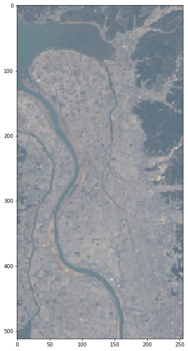
人間の目で見たものと同じような画像を上記のように作成することができまして。それでは、植生指数(NDVI)を導く関数を定義しましょう。NDVIについては「課題に応じて変幻自在? 衛星データをブレンドして見えるモノ・コト」をご覧ください。
def calc_ndvi(red, nir):
	red_float = red.astype(np.float32)
	nir_float = nir.astype(np.float32)
	# calculate NDVI
	# (IR-R)/(IR+R)
	numerator = (nir_float - red_float)
	denominator = (nir_float + red_float)
	flat_numerator = numerator.flatten()
	flat_denominator = denominator.flatten()
	with np.errstate(divide='ignore',invalid='ignore'):
    	ndvi =  np.where(flat_denominator != 0, flat_numerator / flat_denominator, np.nan)
	return ndvi
(2)NDVI(正規化植生指数)を算出する
まずは2014年の4月のデータに対して計算をします。
# rにband4(visible red lightを指定)
r_Apr201401 = get_landsat_blend(Apr2014_land['path'],Apr2014_land['row'],\
                      	Apr2014_land['productId'],12,3645,1535,r=4,g=3,b=2)[:,:,0]
# rにband5(NIRを指定)
nir_Apr201401 = get_landsat_blend(Apr2014_land['path'],Apr2014_land['row'],\
                        	Apr2014_land['productId'],12,3645,1535,r=5,g=3,b=2)[:,:,0]

Apr2014_land_ndvi1 = calc_ndvi(r_Apr201401,nir_Apr201401)
print(Apr2014_land_ndvi1)

# rにband4(visible red lightを指定)
r_Apr201402 = get_landsat_blend(Apr2014_land['path'],Apr2014_land['row'],\
                      	Apr2014_land['productId'],12,3645,1536,r=4,g=3,b=2)[:,:,0]
# rにband5(NIRを指定)
nir_Apr201402 = get_landsat_blend(Apr2014_land['path'],Apr2014_land['row'],\
                        	Apr2014_land['productId'],12,3645,1536,r=5,g=3,b=2)[:,:,0]

Apr2014_land_ndvi2 = calc_ndvi(r_Apr201402,nir_Apr201402)
print(Apr2014_land_ndvi2)

計算された結果を二次元配列に直します。二つの配列を結合し、再び同じ画像を描写してみましょう。
Apr2014_land_ndvi1_wb = Apr2014_land_ndvi1.reshape(256,256)
Apr2014_land_ndvi2_wb = Apr2014_land_ndvi2.reshape(256,256)
Apr2014_land_ndvi_wb_stack = np.vstack((Apr2014_land_ndvi1_wb,Apr2014_land_ndvi2_wb))

plt.figure(figsize = (6,12))
plt.imshow(Apr2014_land_ndvi_wb_stack)
plt.colorbar()
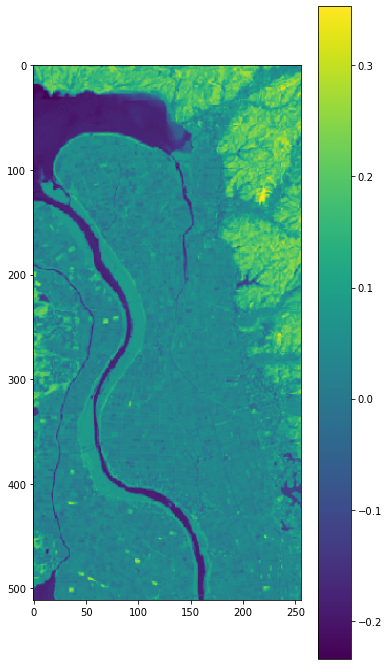
無事、NDVIデータを取得することができました。NDVI値から水面が最も暗く、樹林帯が最も明るい色で表示されていることがわかります。
青森北部では5月の中旬から下旬にかけてが一般的な田植えの時期。この時期にはまだ水も張っていないため、草本類が生えていなければ裸地と考えられます。
既出の研究例 や、NASAの説明 に基づき、代かき(田起こしの終わった田んぼに水を張り、土の表面を平らにする作業)前の水田特定のためのNDVIを0.01から0.08と設定します。
def threshold_ndvi(stack_img,min_val,max_val):
	"""閾値から当該のNDVI値を抽出。画像サイズは512*256のみ"""
	stack_img_ext = np.where((stack_img > min_val) & \
                        	(stack_img < max_val), \
                        	stack_img, np.nan)
	stack_img_reshape = stack_img_ext.reshape(512,256)
	return stack_img_reshape

Apr2014_land_ndvi_wb_reshape = threshold_ndvi(Apr2014_land_ndvi_wb_stack,0.01,0.08)
plt.figure(figsize = (6,12))
plt.imshow(Apr2014_land_ndvi_wb_reshape)
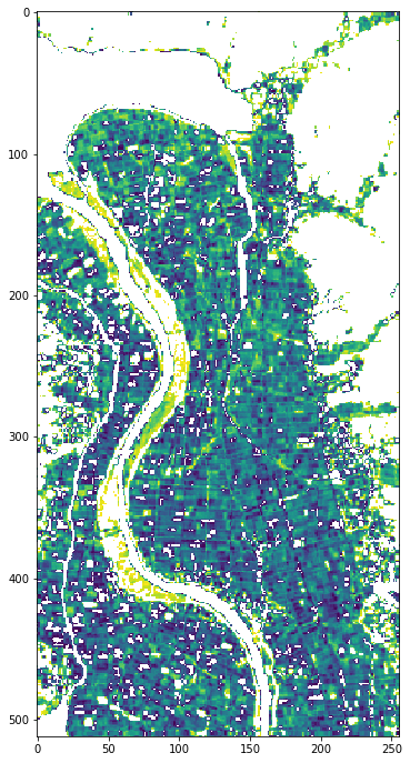
そうすると、上記のような画像になりました。目分量ですが、ある程度分離できたように見えます。続いて、この範囲の水田と指定したNDVI値が画像中にどの程度含まれているのかを計算してみます。
with np.errstate(invalid='ignore'):
	Apr2014_land_ndvi_sum =  np.where((Apr2014_land_ndvi_wb_stack > 0.01) & (Apr2014_land_ndvi_wb_stack < 0.08), 1, 0)
sum(Apr2014_land_ndvi_sum.flatten())/len(Apr2014_land_ndvi_sum.flatten())
結果、おおよそ60%が水田であると見積もることができました。同様のことを2019年の4月のデータに対しても行います。まずは画像を見てみましょう。
# rにband4(visible red lightを指定)
r_Apr201901 = get_landsat_blend(Apr2019_land['path'],Apr2019_land['row'],\
                      	Apr2019_land['productId'],12,3645,1535,r=4,g=3,b=2)[:,:,0]
# rにband5(NIRを指定)
nir_Apr201901 = get_landsat_blend(Apr2019_land['path'],Apr2019_land['row'],\
                        	Apr2019_land['productId'],12,3645,1535,r=5,g=3,b=2)[:,:,0]

Apr2019_land_ndvi1 = calc_ndvi(r_Apr201901,nir_Apr201901)

# rにband4(visible red lightを指定)
r_Apr201902 = get_landsat_blend(Apr2019_land['path'],Apr2019_land['row'],\
                      	Apr2019_land['productId'],12,3645,1536,r=4,g=3,b=2)[:,:,0]
# rにband5(NIRを指定)
nir_Apr201902 = get_landsat_blend(Apr2019_land['path'],Apr2019_land['row'],\
                        	Apr2019_land['productId'],12,3645,1536,r=5,g=3,b=2)[:,:,0]

Apr2019_land_ndvi2 = calc_ndvi(r_Apr201902,nir_Apr201902)

Apr2019_land_ndvi1 = Apr2019_land_ndvi1.reshape(256,256)
Apr2019_land_ndvi2 = Apr2019_land_ndvi2.reshape(256,256)
Apr2019_land_ndvi_wb_stack = np.vstack((Apr2019_land_ndvi1,Apr2019_land_ndvi2))

plt.figure(figsize = (6,12))
plt.imshow(Apr2014_land_ndvi_wb_stack)
plt.colorbar()

先ほどと同様の画像を作成できました。二つの画像を目で比べてみても、大きな違いはないように見えます。次に、閾値を設定したうえで表示すると以下のようになります。
Apr2019_land_ndvi_wb_reshape = threshold_ndvi(Apr2019_land_ndvi_wb_stack,0.01,0.08)
plt.figure(figsize = (6,12))
plt.imshow(Apr2019_land_ndvi_wb_reshape)
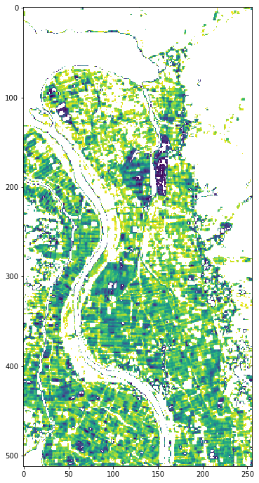
同じ閾値でデータを分類したところ、2019年の方が水田の抽出率が悪いようです。実際に数値で確かめてみましょう。
with np.errstate(invalid='ignore'):
	Apr2019_land_ndvi_sum =  np.where((Apr2019_land_ndvi_wb_stack > 0.01) & (Apr2019_land_ndvi_wb_stack < 0.08), 1, 0)
sum(Apr2019_land_ndvi_sum.flatten())/len(Apr2019_land_ndvi_sum.flatten())
50%程度が水田だと求められました。
(3)指定した範囲のデータを抽出する
今の作業では、取得したタイル画像内の全ての水田(と思しき部分)を抽出してしまっています。そのため、中泊町で米の生産量がどうなったのか、という比較ができません。なので、中泊町の範囲で画像を切り取る必要があります。
行政区域のデータは国土数値情報から入手ができ、国土数値情報行政区域データ青森県N03-110331_02を上のリンクからダウンロードしてみましょう。具体的なダウンロード方法については、別記事をご参照ください。
ダウンロードしたファイルは開発環境の~/work/dataに保存します。
basepath = os.path.expanduser('~')
filepath = basepath + '/work/data/N03-19_02_190101.geojson'
# GeoJSONファイルから、属性データの読み込み
with open(filepath) as f:
	df = json.load(f)
# 中泊町を抽出
nakadomari_features = [f for f in df['features'] if f['properties']['N03_004']=='中泊町']
print(len(nakadomari_features))
print(nakadomari_features[0])
入手したGeoJSONファイルは青森県の全ての市町村データを含んでいます。ここから中泊町だけを選択し、新しいリストに代入しました。実際に区分を表示してみます。
from descartes import PolygonPatch
fig = plt.figure(figsize = (6,12))
ax = fig.gca()
ax.add_patch(PolygonPatch(nakadomari_features[0]['geometry'], fc="#cccccc", ec="#cccccc", alpha=0.5, zorder=2 ))
ax.axis('scaled')
plt.show()
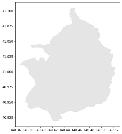
この画像を作成したNDVI画像と重ね合わせることができれば、正確な範囲で切り取ることができます。先ずは、以下の関数を定義しましょう。
タイル画像にはタイル座標の値が含まれていますが、緯度経度の情報が入っているわけではありません。行政区域と重ね合わせるためには、タイル座標を緯度経度に変換する必要があります。座標やタイルの変換における詳しい話はこちらをご覧ください。
from skimage.draw import polygon
def get_tile_bbox(zoom, topleft_x, topleft_y, size_x=1, size_y=1):
	"""
	タイル座標からバウンディングボックスを取得
	https://tools.ietf.org/html/rfc7946#section-5
	"""
	def num2deg(xtile, ytile, zoom):
    	# https://wiki.openstreetmap.org/wiki/Slippy_map_tilenames#Python
    	n = 2.0 ** zoom
    	lon_deg = xtile / n * 360.0 - 180.0
    	lat_rad = math.atan(math.sinh(math.pi * (1 - 2 * ytile / n)))
    	lat_deg = math.degrees(lat_rad)
    	return (lon_deg, lat_deg)
	right_top = num2deg(topleft_x + size_x , topleft_y, zoom)
	left_bottom = num2deg(topleft_x, topleft_y + size_y, zoom)
	return (left_bottom[0], left_bottom[1], right_top[0], right_top[1])
行政区域のGeoJSONファイルには、緯度経度を示すための値が含まれています。ポリゴンはその緯度経度の情報を持ち、上図のように区域を描画することができます。作成した画像はピクセルデータしか持っていません。そのため、このポリゴンの情報をピクセルの情報に置き換える必要があります。
def get_polygon_image(points, bbox, img_size):
	"""
	bboxの領域内にpointsの形状を描画した画像を作成する
	"""
	def lonlat2pixel(bbox, size, lon, lat):
    	"""
    	経度緯度をピクセル座標に変換
    	"""
    	dist = ((bbox[2] - bbox[0])/size[0], (bbox[3] - bbox[1])/size[1])
    	pixel = (int((lon - bbox[0]) / dist[0]), int((bbox[3] - lat) / dist[1]))
    	return pixel
	pixels = []
	for p in points:
    	pixels.append(lonlat2pixel(bbox, (img_size['width'], img_size['height']), p[0], p[1]))
	pixels = np.array(pixels)
	poly = np.ones((img_size['height'], img_size['width']), dtype=np.uint8)
	rr, cc = polygon(pixels[:, 1], pixels[:, 0], poly.shape)
	poly[rr, cc] = 0
	return poly
最後に、ポリゴンの範囲内だけのピクセル情報を抜き出す関数を定義します。
def get_mask_image(features, bbox, px_size):
	"""
	図形からマスク画像を作成する
	Parameters
	----------
	features : array of GeoJSON feature object
    	マスクするfeature objectの配列
	bbox : array
    	描画領域のバウンディングボックス
	px_size : array
    	描画領域のピクセルサイズ
	Returns
	-------
	img_array : ndarray
    	マスク画像
	"""
	ims = []
	for i in range(len(features)):
    	points = features[i]['geometry']['coordinates'][0]
    	ims.append(get_polygon_image(points, bbox, px_size))
	mask = np.where((ims[0] > 0), 0, 1)
	for i in range(1,len(ims)):
    	mask += np.where((ims[i] > 0), 0, 1)
	return np.where((mask > 0), 0, 1).astype(np.uint8)
関数を実行して、中泊町のみを抽出した画像を表示してみましょう。
bbox = get_tile_bbox(12, 3645, 1535, 1, 2)
px_size = {'width': Apr2019_land_ndvi_wb_stack.shape[1], 'height': Apr2019_land_ndvi_wb_stack.shape[0]}
nakadomari_features_mask = get_mask_image(nakadomari_features, bbox, px_size)
plt.figure(figsize = (6,12))
io.imshow(nakadomari_features_mask)
中泊町以外は黄色く表示されているのがわかります。
この画像とAPIで取得した画像を利用して、マスキングされた画像を作成します。
Apr2014_mask_img = np.where(nakadomari_features_mask != 1, Apr2014_land_ndvi_wb_stack, 0)
plt.figure(figsize = (6,12))
plt.imshow(Apr2014_mask_img)
plt.colorbar()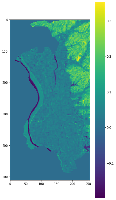
中泊町の範囲だけが切り取られました。この範囲内で、先ほどと同様の条件で水田を抽出してみます。
with np.errstate(invalid='ignore'):
	Apr2014_mask_img_sum =  np.where((Apr2014_mask_img > 0.01) & (Apr2014_mask_img < 0.08), 1, 0)
sum(Apr2014_mask_img_sum.flatten())/len(Apr2014_mask_img_sum.flatten())
# 0.374542236328125
約4割が水田であることが示されました。2019年のデータでも同様の処理を行います。
Apr2019_mask_img = np.where(nakadomari_features_mask != 1, Apr2019_land_ndvi_wb_stack, 0)
plt.figure(figsize = (6,12))
plt.imshow(Apr2019_mask_img)
plt.colorbar()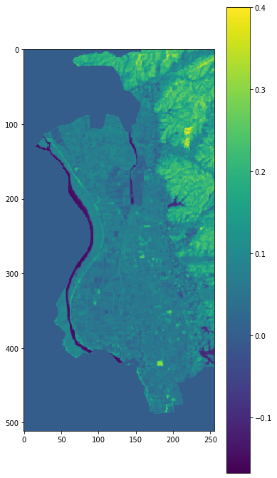
with np.errstate(invalid='ignore'):
	Apr2019_mask_img_sum =  np.where((Apr2019_mask_img > 0.01) & (Apr2019_mask_img < 0.08), 1, 0)
sum(Apr2019_mask_img_sum.flatten())/len(Apr2019_mask_img_sum.flatten())
# 0.29027557373046875
約3割が水田であると示されました。
さらに、二つの画像から差分をとって、具体的にどの部分が水田でないと判断されたのかを確認しましょう。
(4)水田の差を比較する
# 2014年と2019年の差分画像を作成する
diff_ndvi = Apr2014_mask_img_sum - Apr2019_mask_img_sum
# 2019年では水田でなくなった部分を抽出
diff_ndvi_ext = np.where(diff_ndvi==1,1,0)
plt.figure(figsize = (6,12))
plt.imshow(diff_ndvi_ext)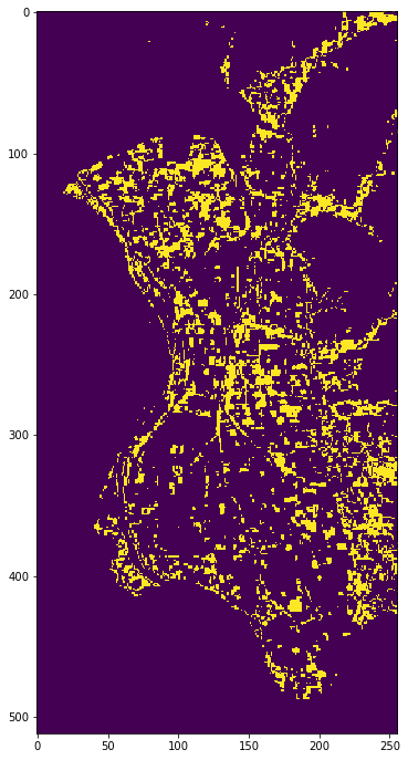
黄色い部分が2019年では水田と判断されなかった箇所になります。
2014年と2019年のデータを比較したところ、取得したシーン内の中泊町のエリアでも約1割程度の水田がなくなったと予想される結果となりました。
後編では実際に政府統計データとの突き合わせを実施し、衛星データで算出したデータの傾向とに乖離があるのか確認します。