ペア画像必要なし!教師なし学習で光学画像とSAR画像を相互変換する
本稿では、公開されているデータセットを利用し、ペア画像を必要としない教師なし学習によって「光学画像→SAR画像変換、及びSAR画像→光学画像変換」を実現します。
2022年8月31日以降、Tellus OSでのデータの閲覧方法など使い方が一部変更になっております。新しいTellus OSの基本操作は以下のリンクをご参照ください。
https://www.tellusxdp.com/ja/howtouse/tellus_os/start_tellus_os.html
1. はじめに
本稿では以下のように「光学画像→SAR画像変換、及びSAR画像→光学画像変換」をペア画像を必要としない教師なし学習で実現します。
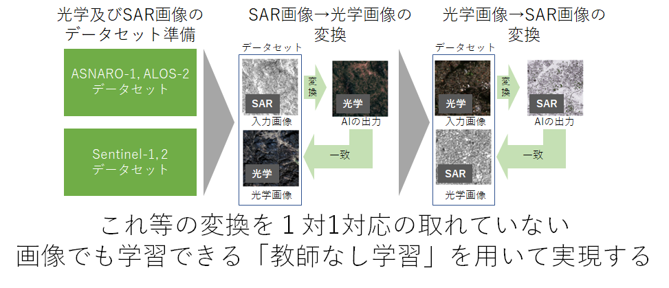
SARは天候に左右されることなく地球を可視できるため、その需要は年々増加の一途を辿っています。しかし、SARは主に衛星や航空機でのみ用いられている特殊なセンサであるため、未だデータ数が少なく、またデータ取得コストも非常に高いといった課題があります。また、SARは一般的な光学カメラとは異なり、電磁波による観測のためシミュレーションも非常に難しく、大量のデータが必要となる機械学習と相性が悪いといった課題もあります。
これに対して、既に様々な方々が光学画像からSAR画像を生成したり、またはその逆にSAR画像を光学化したりするといったことを、教師あり機械学習を用いて行っています。しかし、これにも課題が残ります。それは、光学及びSAR画像で一対一対応が取れるペア画像を用意することが非常に難しいということです。一対一対応とは、画像内の同じ位置に同じ対象物が同じ撮影条件で映っている状態を表します。理想的な高品質のペア画像を得るためには、ある衛星にSAR及び光学の両センサが搭載されており、2つの解像度や仕様が概ね同じであり、かつ同時に観測を行い、そのデータが公開されている必要があります。この条件を満たすのは今日では難しいでしょう。仮に、この条件を満たした光学及びSARの画像があったとしても、それらのマッチング処理(微小な位置合わせや同じ観測条件の抽出)を行うことは大変です。
一方、「異なる衛星間で、きちんとしたマッチング処理もしなくて良い」という条件であれば、近しい場所を異なる解像度、オフナディア角等で観測したSAR及び光学の画像はあります。例えば、ASNARO-1(光学画像)及びALOS-2(SAR画像)等のペアが挙げられます。ただし、これら2つの衛星は、画像としての仕様がそもそも異なるため、高品質なペア画像とならず、教師あり学習は難しいでしょう。
そこで今回は、教師なし学習を用いて「高品質なペア画像を用いずとも光学↔SAR画像の相互変換を達成する」ことに挑戦したいと思います。
本稿で挑戦することは以下です。
・ASNARO-1(光学画像)及びALOS-2(SAR画像)のデータを雑に集めて、光学↔SAR画像の相互変換を行う
・ある程度高品質な光学及びSARのペア画像(Sentinel-1, 2)を用いて光学↔SAR画像変換を行う
・光学↔SAR画像変換は教師なし(CycleGAN)、教師あり(Pix2Pix)学習の両方で行い、その違いを比較する
2. 変換アルゴリズムの技術紹介
今回は教師あり学習にPix2Pix、教師なし学習にCycleGANといった機械学習のアルゴリズムを用います。これら2つの技術は主にテクスチャ(物体の構造ではなく表面のパターンや色合い)の変換を目的としており、基盤技術にGAN(Generative Adversarial Networks)と呼ばれるものが共通して用いられています。
Pix2PixやGANについては「SAR画像から光学画像への変換をpix2pixで実装して、作った生成器で別のSAR画像を分析してみた」で詳しく解説しているので説明は割愛し、本稿ではCycleGanに絞って説明します。
CycleGAN(https://arxiv.org/abs/1703.10593)の際立った特徴としては、教師なし学習により2つの画像間の相互テクスチャ変換を実現したことです。これをドメイン変換といいます。
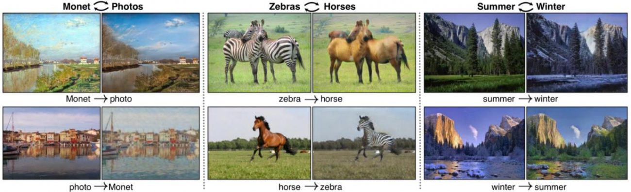
こちらは論文から引用した、CycleGanを用いた最も有名な画像である「シマウマ↔ウマ」の変換の例です。ウマという共通の形状を残しながら、テクスチャのみを変換しています。これは光学画像をSAR画像へ変換する際の「大きな構造は変化させず見え方(テクスチャ)だけを変える」といった部分に通ずる点です。
論文中の図を基に、その仕組みを詳しく説明していきましょう。
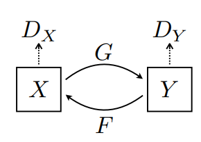
Xはシマウマのデータセット、すなわちシマウマドメインだと考えて下さい。次にYはウマのデータセット、すなわちウマドメインだと考えて下さい。このとき、Gはシマウマをウマに変換する装置と考えてください。Fはその逆で、ウマをシマウマに変換する装置のことです。これら変換結果が正しいものなのか否かについて判断する機会が、GANでいうところのDiscriminaterと呼ばれるDx、Dyです。
最適化された状態を考えるとG(F(Y))=Yとなります。これはつまり、ウマをシマウマに変換でき、かつシマウマはウマに変換できる状態において、元の入力したウマと変換したウマが一致するため、入力と出力が循環します。このため、サイクルGANと呼ばれています。換言すると、シマウマ=F(ウマ)、ウマ=G(シマウマ)の時、G(F(ウマ))=ウマとなり、入力と出力が循環一致するということです。
これは2つのドメイン(分布)の差異を打ち消すような2つの機械(G, F)を作ることができれば、光学↔SAR画像の相互変換を行うことができると考えて下さい。これを教師なしで学習させるため、様々な損失関数を組み合わせていますが、ここでは詳細説明は割愛します。興味ある方は論文を読んでみてください。
3. データセットの準備
今回は以下2つのデータセットを準備します。
1) 高品質な光学及びSARのペア画像(Sentinel-1, 2)
2) ASNARO-1(光学画像)及びALOS-2(SAR画像)のデータ
3.1. 高品質な光学とSARのペア画像(Sentinel-1, 2)
1つ目はSentinel-1(SAR)及びSentinel-2(光学)衛星によって観測された画像を幾何学一致させたデータセットです。以下からダウンロードできます。
https://mediatum.ub.tum.de/1436631
全てダウンロードすると45GB程度と膨大なので、今回は「ROIs1970_fall」フォルダの中から一部を選択して使います。
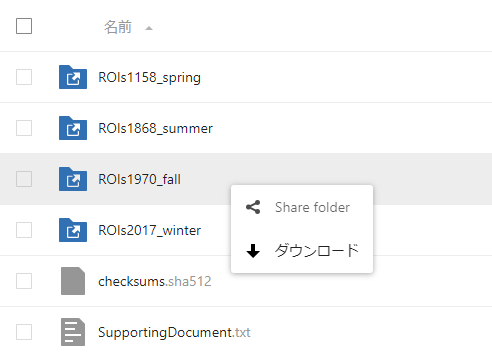
開発環境上にダウンロードが完了したら以下を実行してデータを解凍しましょう。
$ unzip ROIs1970_fall
解凍すると「s1_1、s1_2、s1_3…、s2_1、s2_2、s2_3…」とフォルダが続きます。これらは、s1がSAR画像、s2が光学画像となっており、それ以外のファイル名は殆ど一致しています。各画像は256pxで統一されており、SARはVV偏波の画像となっています。
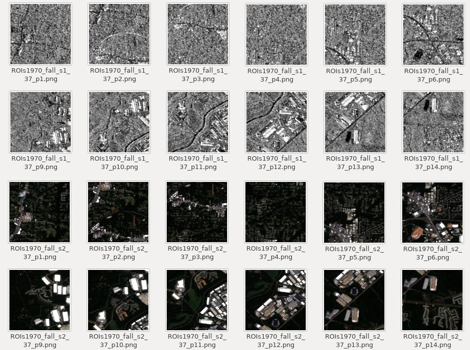
これらは光学及びSARのペア画像としてかなり品質の高いデータであり、これなら相互変換も達成できそうです。
現状、ペアになっているので、教師なし学習として利用するために、ペアを解消して使います。
3.2. ASNARO-1(光学画像)、ALOS-2(SAR画像)のデータ
次に2つ目のデータはTellusの環境から自前で構築していきます。まずはスカイツリー周辺のALOS-2のSAR L2.1画像を得ます。
import os, requests
import geocoder # ! pip install geocoder

# Fields
BASE_API_URL = "https://file.tellusxdp.com/api/v1/origin/search/" # https://www.tellusxdp.com/docs/api-reference/palsar2-files-v1.html#/
ACCESS_TOKEN = "ご自身のトークンを貼り付けてください"
HEADERS = {"Authorization": "Bearer " + ACCESS_TOKEN}
TARGET_PLACE = "Skytree, Tokyo"
SAVE_DIRECTORY="./data/"

# Functions
def rect_vs_point(ax, ay, aw, ah, bx, by):
    return 1 if bx > ax and bx  ay and by < ah else 0

def get_scene_list(_get_params={}):
    query = "palsar2-l21"
    r = requests.get(BASE_API_URL + query, _get_params, headers=HEADERS)
    if not r.status_code == requests.codes.ok:
        r.raise_for_status()
    return r.json()

def get_scenes(_target_json, _get_params={}):
    # get file list
    r = requests.get(_target_json["publish_link"], _get_params, headers=HEADERS)
    if not r.status_code == requests.codes.ok:
        r.raise_for_status()
    file_list = r.json()['files']
    dataset_id = _target_json['dataset_id'] # folder name
    # make dir
    if os.path.exists(SAVE_DIRECTORY + dataset_id) == False:
        os.makedirs(SAVE_DIRECTORY + dataset_id)
    # downloading
    print("[Start downloading]", dataset_id)
    for _tmp in file_list:
        r = requests.get(_tmp['url'], headers=HEADERS, stream=True)
        if not r.status_code == requests.codes.ok:
            r.raise_for_status()
        with open(os.path.join(SAVE_DIRECTORY, dataset_id, _tmp['file_name']), "wb") as f:
            f.write(r.content)
        print("  - [Done]", _tmp['file_name'])
    print("finished")
    return

# Entry point
def main():
    # extract slc list around the address
    gc = geocoder.osm(TARGET_PLACE, timeout=5.0) # get latlon
    #print(gc.latlng)
    scene_list_json = get_scene_list({"page_size":"1000", "mode":"SM1", "left_bottom_lat":  gc.latlng[0], "left_bottom_lon":  gc.latlng[1], "right_top_lat":  gc.latlng[0], "right_top_lon":  gc.latlng[1]})
    #print(scene_list_json["count"])
    target_places_json = [_ for _ in scene_list_json['items'] if rect_vs_point(_['bbox'][1], _['bbox'][0], _['bbox'][3], _['bbox'][2], gc.latlng[0], gc.latlng[1])] # lot_min, lat_min, lot_max...
    #print(target_places_json)
    target_ids = [_['dataset_id'] for _ in target_places_json]
    print("[Matched SLCs]", target_ids)
    # download
    for target_id in target_ids:
        target_json = [_ for _ in scene_list_json['items'] if _['dataset_id'] == target_id][0]
        # download the target file
        get_scenes(target_json)

if __name__=="__main__":
       main()
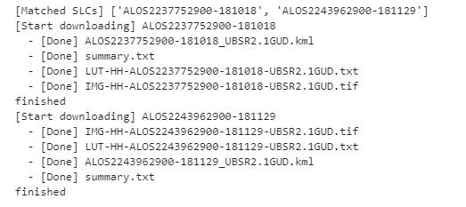
実行すると以下2つが該当し、dataフォルダに保存されます。
コードの特に重要な部分のみ説明します。
scene_list_json = get_scene_list({"page_size":"1000", "mode":"SM1", "left_bottom_lat": gc.latlng[0], "left_bottom_lon": gc.latlng[1], "right_top_lat": gc.latlng[0], "right_top_lon": gc.latlng[1]})この部分でTellusのAPIを叩き、条件に一致するSAR画像があるかを確認しています。条件にはスカイツリーが画像に含まれていること、またSM1であることを設定しています。SM1はStripmap1というSAR観測のモードで3m分解能のものを指します。ダウンロードしたSAR画像はGeoTiffといってピクセル値に加えて緯度経度情報も持っています。
次に、ダウンロードしたこのSAR画像から特定域のみを抽出します。そのためには、緯度経度を用いて画像を切り抜くのですが、ダウンロードしたGeoTiffは$gdalinfoでファイルの表示形式を調べると以下のように「ESPG:9001」となっています。
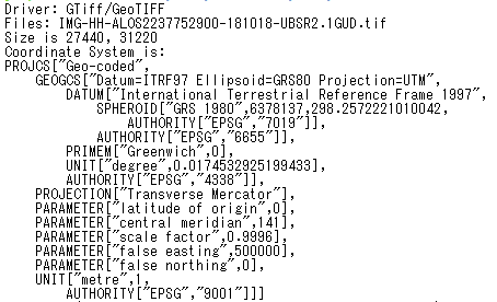
GDALというGeoTiff等の処理に特化したソフトウェアを用いて、緯度経度からGeoTiff画像を切り抜くことがこのファイル形式のままでは難しいため、以下のプログラムでEPSG:9001➔EPSG:4326の投影方式の変換及び緯度経度による画像の切り抜きを行います。
import os, requests, subprocess
from osgeo import gdal
from osgeo import gdal_array

# Entry point
def main():
    cmd = "find ./data/ALOS* | grep tif"
    process = (subprocess.Popen(cmd, stdout=subprocess.PIPE,shell=True).communicate()[0]).decode('utf-8')
    file_name_list = process.rsplit()
    for _file_name in file_name_list:
        convert_file_name =   _file_name + "_converted.tif"
        crop_file_name =   _file_name + "_cropped.tif"
        x1 = 139.807069
        y1 = 35.707233
        x2 = 139.814111
        y2 = 35.714069
        cmd = 'gdalwarp -t_srs EPSG:4326 ' +_file_name + ' ' + convert_file_name
        process = (subprocess.Popen(cmd, stdout=subprocess.PIPE,shell=True).communicate()[0]).decode('utf-8')
        print("[Done] ", convert_file_name)
        cmd = 'gdal_translate -projwin ' + str(x1) + ' ' + str(y1) + ' ' +  str(x2) + ' ' + str(y2) + ' ' + convert_file_name + " " + crop_file_name
        print(cmd)
        process = (subprocess.Popen(cmd, stdout=subprocess.PIPE,shell=True).communicate()[0]).decode('utf-8')
        print("[Done] ", crop_file_name)

if __name__=="__main__":
       main()
これら処理が完了すると次のようなファイルが揃います。

今回使うデータは~cropped.tifとなっているものです。
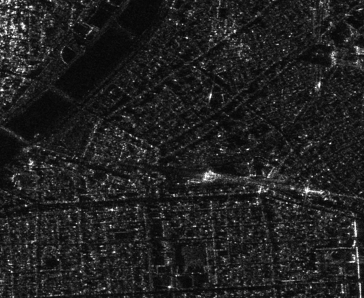
スカイツリー周辺域が切り抜かれているSAR画像を得ることができました。
では、重要な部分のみコードを説明します。
以下はGDALというソフトウェアを用いて座標系の変換をしています。
cmd = 'gdalwarp -t_srs EPSG:4326 ' +_file_name + ' ' + convert_file_name続いて、以下でもGDALというソフトウェアを用いてスカイツリー周辺域の緯度経度から画像を切り抜いています。
cmd = 'gdal_translate -projwin ' + str(x1) + ' ' + str(y1) + ' ' + str(x2) + ' ' + str(y2) + ' ' + convert_file_name + " " + crop_file_nameここまででSAR画像の準備はできました。次に、スカイツリー周辺域を切り抜いたSAR画像に一致する光学画像をASNARO-1から探します。まずは以下のコードを実行してください。
import os, requests
import geocoder # ! pip install geocoder
import math
from skimage import io
from io import BytesIO
import numpy as np
import cv2

# Fields
BASE_API_URL = "https://gisapi.tellusxdp.com"
ASNARO1_SCENE = "/api/v1/asnaro1/scene"
ACCESS_TOKEN = "ご自身のトークンを貼り付けてください"
HEADERS = {"Authorization": "Bearer " + ACCESS_TOKEN}
TARGET_PLACE = "skytree, Tokyo"
SAVE_DIRECTORY="./data/asnaro/"
ZOOM_LEVEL=18
IMG_SYNTH_NUM=6
IMG_BASE_SIZE=256

# Functions
def get_tile_num(lat_deg, lon_deg, zoom):
    lat_rad = math.radians(lat_deg)
    n = 2.0 ** zoom
    xtile = int((lon_deg + 180.0) / 360.0 * n)
    ytile = int((1.0 - math.log(math.tan(lat_rad) + (1 / math.cos(lat_rad))) / math.pi) / 2.0 * n)
    return (xtile, ytile)

def get_scene_list(_get_params={}):
    query = BASE_API_URL + ASNARO1_SCENE
    r = requests.get(query, _get_params, headers=HEADERS)
    if not r.status_code == requests.codes.ok:
        r.raise_for_status()
    return r.json()

def get_scene(_id, _xc, _yc):
    # mkdir
    save_file_name = SAVE_DIRECTORY + _id + ".png"
    if os.path.exists(SAVE_DIRECTORY) == False:
        os.makedirs(SAVE_DIRECTORY)

    # download
    save_image = np.zeros((IMG_SYNTH_NUM * IMG_BASE_SIZE, IMG_SYNTH_NUM * IMG_BASE_SIZE, 3))
    for i in range(IMG_SYNTH_NUM):
        for j in range(IMG_SYNTH_NUM):
            query = "/ASNARO-1/" + _id + "/" + str(ZOOM_LEVEL) + "/" + str(_xc-int(IMG_SYNTH_NUM*0.5)+i) + "/" + str(_yc-int(IMG_SYNTH_NUM*0.5)+j) + ".png"
            r = requests.get(BASE_API_URL + query, headers=HEADERS)
            if not r.status_code == requests.codes.ok:
                r.raise_for_status()
            img = io.imread(BytesIO(r.content))
            save_image[i*IMG_BASE_SIZE:(i+1)*IMG_BASE_SIZE, j*IMG_BASE_SIZE:(j+1)*IMG_BASE_SIZE, :] = img[:, :, 0:3].transpose(1, 0, 2) # [x, y, c] -> [y, x, c]
    save_image = cv2.flip(save_image, 1)
    save_image = cv2.rotate(save_image, cv2.ROTATE_90_COUNTERCLOCKWISE)
    cv2.imwrite(save_file_name, save_image)
    print("[DONE]" + save_file_name)
    return


# Entry point
def main():
    # extract slc list around the address
    gc = geocoder.osm(TARGET_PLACE, timeout=5.0) # get latlon
    scene_list = get_scene_list({"min_lat":  gc.latlng[0], "min_lon":  gc.latlng[1], "max_lat":  gc.latlng[0], "max_lon":  gc.latlng[1]})
    for _scene in scene_list:
        #_xc, _yc = get_tile_num(_scene['clat'], _scene['clon'], ZOOM_LEVEL) # center
        _xc, _yc = get_tile_num(gc.latlng[0], gc.latlng[1], ZOOM_LEVEL)
        get_scene(_scene['entityId'], _xc, _yc)

if __name__=="__main__":
       main()
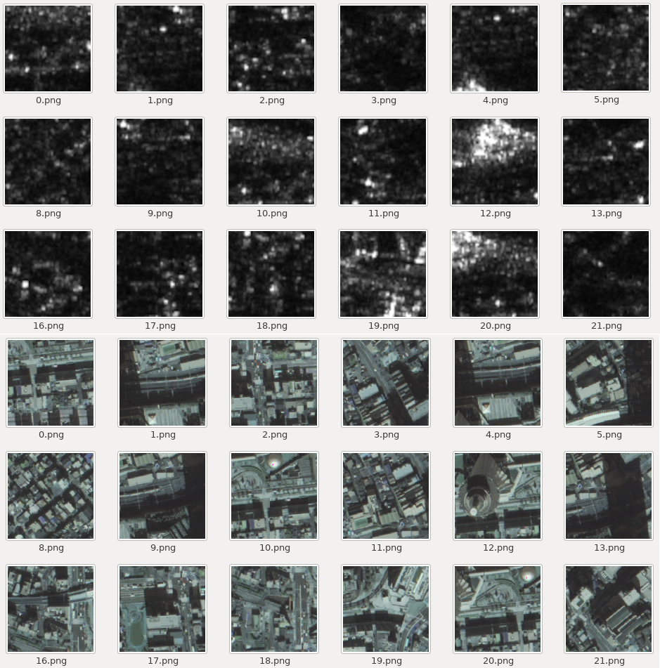
これを実行すると以下のような結果が得られます。
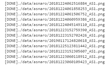
これはASNARO-1が保有する観測データからスカイツリー周辺域を抽出してきたものになります。ASNARO-1のAPIはTellusの制約上パッチ画像しか得られないため、スカイツリー周辺域の画像がありそうなものを検索して探してきた後に、その周辺のパッチを集めて合成するという処理を行っています。このため、高解像度で広域の一枚画像を以下のように得ることができています。
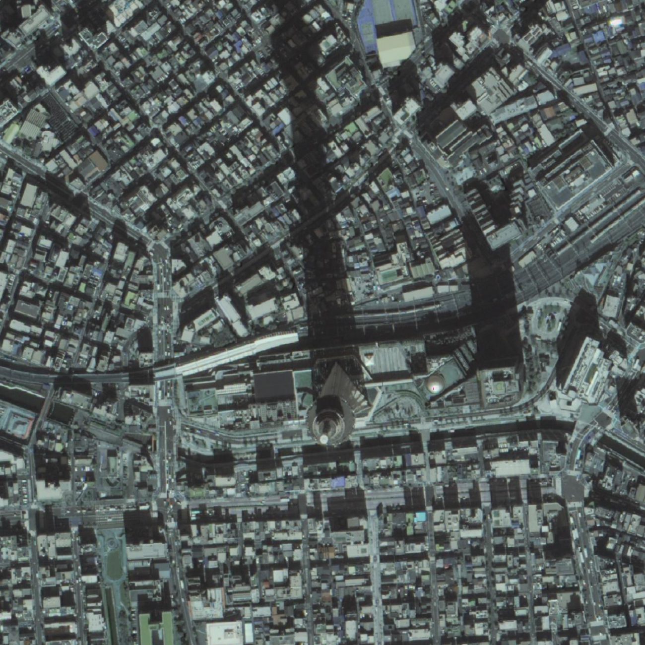
角度によってはスカイツリーが倒れ込んでしまっている画像もあるので、見た目で倒れこみやブラー(ボケ)、ノイズ等がなさそうな画像を選びます。
では重要な部分のみコードを説明します。
以下からスカイツリーが観測されているASNARO-1の観測データリストを得ています。
scene_list = get_scene_list({"min_lat": gc.latlng[0], "min_lon": gc.latlng[1], "max_lat": gc.latlng[0], "max_lon": gc.latlng[1]})以下でスカイツリー周辺域のパッチ画像を集めて一枚の画像にしています。
        _xc, _yc = get_tile_num(gc.latlng[0], gc.latlng[1], ZOOM_LEVEL)
        get_scene(_scene['entityId'], _xc, _yc)
get_scene関数の中では以下の処理が奇妙に思うかもしれません。
            save_image[i*IMG_BASE_SIZE:(i+1)*IMG_BASE_SIZE, j*IMG_BASE_SIZE:(j+1)*IMG_BASE_SIZE, :] = img[:, :, 0:3].transpose(1, 0, 2) # [x, y, c] -> [y, x, c]
    save_image = cv2.flip(save_image, 1)
    save_image = cv2.rotate(save_image, cv2.ROTATE_90_COUNTERCLOCKWISE)
これは、得られたパッチ画像の配列がx, y, cであるものの、OpenCVで書き出す場合はy, x, cとして扱わなければならないため、その変換処理が書かれています。また、SAR画像と同じノースアップとなるよう回転処理が加えられています。
これで2つの光学及びSAR画像が揃いました。このままでも機械学習に入力することはできますが、その出力を人間が目で判断した時に合っているか間違っているか理解できるように、一応不格好ながらもマッチング処理もしておきます。
ALOS-2のSAR画像の分解能は3m、ASNARO-1のマルチ画像の分解能は2mで、それぞれ撮像条件やオフナディア角も違います。このため、完全一致は不可能で、雑にそれらしく位置を合わせる簡易的なマッチング処理を行います。
マッチング処理は以下のコードを実行します。(参考: https://qiita.com/suuungwoo/items/9598cbac5adf5d5f858e)今回使用するAKAZEという手法は2つの画像間のスケール、回転、シフトの差異全てに対応している、優れているマッチング処理アルゴリズムです。
import cv2

float_img = cv2.imread('data/ALOS2237752900-181018/IMG-HH-ALOS2237752900-181018-UBSR2.1GUD.tif_cropped.tif', cv2.IMREAD_GRAYSCALE)
ref_img = cv2.imread('data/asnaro/20181224060959386_AS1.png', cv2.IMREAD_GRAYSCALE)

akaze = cv2.AKAZE_create()
float_kp, float_des = akaze.detectAndCompute(float_img, None)
ref_kp, ref_des = akaze.detectAndCompute(ref_img, None)
bf = cv2.BFMatcher()
matches = bf.knnMatch(float_des, ref_des, k=2)
good_matches = []
for m, n in matches:
    if m.distance < 0.95 * n.distance:
        good_matches.append([m])

matches_img = cv2.drawMatchesKnn(
    float_img,
    float_kp,
    ref_img,
    ref_kp,
    good_matches,
    None,
    flags=cv2.DrawMatchesFlags_NOT_DRAW_SINGLE_POINTS)
cv2.imwrite('matches.png', matches_img)
実行すると以下のような画像が得られます。
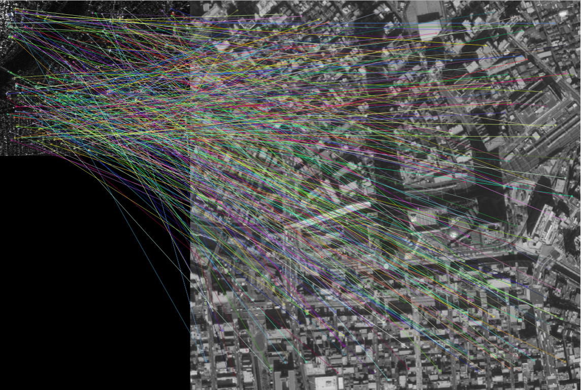
このマッチング情報を基に、地形一致の場所などにあたりを付けて、手動で台形補正等を行い微調整していきます。結果的に以下のような2つのペア画像ができました。
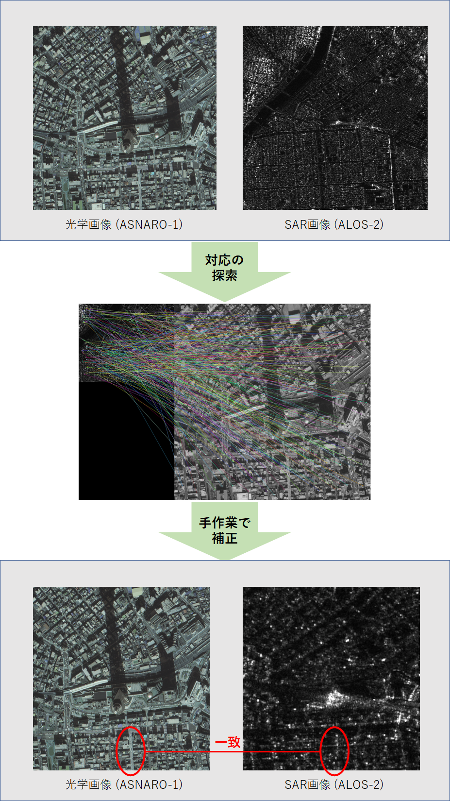
2つの画像を見て、もはや別物だと思うかもしれませんが、道路の位置、大きさ等は一致しています。しかし分解能に大きな違いがあるため、SAR画像の方では建物などの構造物がつぶれてしまっています。
これで以下2つのデータの準備ができました。
- 高品質な光学及びSARのペア画像(Sentinel-1, 2)
- ASNARO-1(光学画像)及びALOS-2(SAR画像)のデータ
次にいよいよ学習をさせていきたいと思います。
4. 教師なし学習(CycleGan)による光学↔SAR画像変換
今回CycleGanの実装は(https://github.com/eriklindernoren/Keras-GAN/tree/master/cyclegan)を参考に実装していきました。
※途中でデータ読み込みのプログラム等、共通的に使うプログラムが出てくるので、飛ばさずにお読みください
4.1. 高品質な光学及びSARのペア画像(SEN-1, 2)
ではまず、頭記のデータセットから試していきたいと思います。
まずは$mkdir your_workfolderで作業フォルダを作成し、以降それをルートディレクトリとして扱い、同一フォルダ内で作業を行ってください。流れに沿ってプログラムを実行していけば最終的には以下と同じディレクトリ構造になるはずです。もし異なっていた場合は手順を再度確認してみて下さい。
root
|- cyclegan.py
|- data_loader_py
|- datasets
| |- sat
| |-testA
| | |- file...
| |-testB
| | |- file...
| |-trainA
| | |- file...
| |-trainB
| |- file...
|- data_split.py
|- images
| |- sar
| |- file…
|- ROIs1970_fall (どこに設置しても良い)
データセットのROIs1970_fallを2つのドメイン(光学及びSAR)の画像に分けるため、以下のコードを実行します。ここではdata_split.pyという名前で保存します。
import os, requests, subprocess
import math
import numpy as np
import cv2
import random

# read dataset
file_path = "./ROIs1970_fall/"
cmd = "find " + file_path + "s1* | grep png"
process = (subprocess.Popen(cmd, stdout=subprocess.PIPE,shell=True).communicate()[0]).decode('utf-8')
file_name_list = process.rsplit()
data_x = []
data_y = []
for _file_name in file_name_list:
  data_x.append(_file_name)
  data_y.append(_file_name.replace('s1_','s2_'))
data_x = np.asarray(data_x)
data_y = np.asarray(data_y)

# extract data
part_data_ratio = 0.1 # extract data depending on the ratio from all data
test_data_ratio = 0.1
all_data_size = len(data_x)
idxs = range(all_data_size) # all data
part_idxs = random.sample(idxs, int(all_data_size * part_data_ratio)) # part data
part_data_size = len(part_idxs)
test_data_idxs = random.sample(part_idxs, int(part_data_size * test_data_ratio)) # test data from part data
train_data_idxs = list(set(part_idxs) - set(test_data_idxs)) # train data = all data - test data
test_x = data_x[test_data_idxs]
test_y = data_y[test_data_idxs]
train_x = data_x[train_data_idxs]
train_y = data_y[train_data_idxs]

# data copy
os.makedirs('datasets/sar/trainA', exist_ok=True)
os.makedirs('datasets/sar/trainB', exist_ok=True)
os.makedirs('datasets/sar/testA', exist_ok=True)
os.makedirs('datasets/sar/testB', exist_ok=True)
cmd = 'find ./datasets/sar/* -type l -exec unlink {} \;'
process = (subprocess.Popen(cmd, stdout=subprocess.PIPE,shell=True).communicate()[0]).decode('utf-8')
print("[Start] extract test dataset")
for i in range(len(test_x)):
  cmd = "ln -s " + test_x[i] + " datasets/sar/testA/"
  process = (subprocess.Popen(cmd, stdout=subprocess.PIPE,shell=True).communicate()[0]).decode('utf-8')
  cmd = "ln -s " + test_y[i] + " datasets/sar/testB/"
  process = (subprocess.Popen(cmd, stdout=subprocess.PIPE,shell=True).communicate()[0]).decode('utf-8')
  if i % 500 == 0:
    print("[Done] ", i, "/", len(test_x))
print("Finished")

print("[Start] extract train dataset")
for i in range(len(train_x)):
  cmd = "ln -s " + train_x[i] + " datasets/sar/trainA/"
  process = (subprocess.Popen(cmd, stdout=subprocess.PIPE,shell=True).communicate()[0]).decode('utf-8')
  cmd = "ln -s " + train_y[i] + " datasets/sar/trainB/"
  process = (subprocess.Popen(cmd, stdout=subprocess.PIPE,shell=True).communicate()[0]).decode('utf-8')
  if i % 500 == 0:
    print("[Done] ", i, "/", len(train_x))
print("Finished")
これを実行すると./datasets/sar/配下に「trainA, trainB, testA, testB」といったフォルダが生成され、各ドメインの画像が分けられます。AがSARドメイン、Bが光学ドメインとなっています。
この生成された画像を読み込むデータローダのプログラムは以下です。data_loader.pyという名前で〇〇の階層にファイルを保存してください。他のプログラムから後ほど参照されることになるので、階層は正しく設置してください。
import scipy
from glob import glob
import numpy as np

class DataLoader():
    def __init__(self, dataset_name, img_res=(256, 256)):
        self.dataset_name = dataset_name
        self.img_res = img_res

    def load_data(self, domain, batch_size=1, is_testing=False):
        data_type = "train%s" % domain if not is_testing else "test%s" % domain
        path = glob('./datasets/%s/%s/*' % (self.dataset_name, data_type))

        batch_images = np.random.choice(path, size=batch_size)

        imgs = []
        for img_path in batch_images:
            img = self.imread(img_path)
            if not is_testing:
                img = scipy.misc.imresize(img, self.img_res)

                if np.random.random() > 0.5:
                    img = np.fliplr(img)
            else:
                img = scipy.misc.imresize(img, self.img_res)
            imgs.append(img)

        imgs = np.array(imgs)/127.5 - 1.
        return imgs

    def load_data_with_label(self, domain, batch_size=1, is_testing=False):
        data_type = "train%s" % domain if not is_testing else "test%s" % domain
        path = glob('./datasets/%s/%s/*' % (self.dataset_name, data_type))

        batch_images = np.random.choice(path, size=batch_size)

        imgs = []
        lbls = []
        for img_path in batch_images:
            img = self.imread(img_path)
            # lbl path
            if "A/" in img_path:
              lbl_path = img_path.replace('s1_', 's2_')
              lbl_path = lbl_path.replace('A/', 'B/')
            else:
              lbl_path = img_path.replace('s2_', 's1_')
              lbl_path = lbl_path.replace('B/', 'A/')
            lbl = self.imread(lbl_path)

            if not is_testing:
                img = scipy.misc.imresize(img, self.img_res)
                lbl = scipy.misc.imresize(lbl, self.img_res)

                if np.random.random() > 0.5:
                    img = np.fliplr(img)
                    lbl = np.fliplr(lbl)
            else:
                img = scipy.misc.imresize(img, self.img_res)
                lbl = scipy.misc.imresize(lbl, self.img_res)
            imgs.append(img)
            lbls.append(lbl)
        imgs = np.array(imgs)/127.5 - 1.
        lbls = np.array(lbls)/127.5 - 1.
        return imgs, lbls


    def load_batch(self, batch_size=1, is_testing=False):
        data_type = "train" if not is_testing else "val"
        path_A = glob('./datasets/%s/%sA/*' % (self.dataset_name, data_type))
        path_B = glob('./datasets/%s/%sB/*' % (self.dataset_name, data_type))

        self.n_batches = int(min(len(path_A), len(path_B)) / batch_size)
        total_samples = self.n_batches * batch_size

        # Sample n_batches * batch_size from each path list so that model sees all
        # samples from both domains
        path_A = np.random.choice(path_A, total_samples, replace=False)
        path_B = np.random.choice(path_B, total_samples, replace=False)

        for i in range(self.n_batches-1):
            batch_A = path_A[i*batch_size:(i+1)*batch_size]
            batch_B = path_B[i*batch_size:(i+1)*batch_size]
            imgs_A, imgs_B = [], []
            for img_A, img_B in zip(batch_A, batch_B):
                img_A = self.imread(img_A)
                img_B = self.imread(img_B)

                img_A = scipy.misc.imresize(img_A, self.img_res)
                img_B = scipy.misc.imresize(img_B, self.img_res)

                if not is_testing and np.random.random() > 0.5:
                        img_A = np.fliplr(img_A)
                        img_B = np.fliplr(img_B)

                imgs_A.append(img_A)
                imgs_B.append(img_B)

            imgs_A = np.array(imgs_A)/127.5 - 1.
            imgs_B = np.array(imgs_B)/127.5 - 1.

            yield imgs_A, imgs_B

    def load_img(self, path):
        img = self.imread(path)
        img = scipy.misc.imresize(img, self.img_res)
        img = img/127.5 - 1.
        return img[np.newaxis, :, :, :]

    def imread(self, path):
        return scipy.misc.imread(path, mode='RGB').astype(np.float)
このプログラムはCycleGanのプログラムが学習を行うたびに呼ばれます。imgs_A及びimgs_BにSAR及び光学の画像が保存されるようになっています。では、いよいよ本体のCycleGanのプログラムです。cyclegan.pyという名前で同一階層に保存してください。
from __future__ import print_function, division
import scipy

from keras.datasets import mnist
from keras_contrib.layers.normalization.instancenormalization import InstanceNormalization
from keras.layers import Input, Dense, Reshape, Flatten, Dropout, Concatenate
from keras.layers import BatchNormalization, Activation, ZeroPadding2D
from keras.layers.advanced_activations import LeakyReLU
from keras.layers.convolutional import UpSampling2D, Conv2D
from keras.models import Sequential, Model
from tensorflow.keras.optimizers import Adam
import datetime
import sys
from data_loader import DataLoader
import numpy as np
import os
import matplotlib as mpl
mpl.use('Agg')
import matplotlib.pyplot as plt

class CycleGAN():
    def __init__(self):
        # Input shape
        self.img_rows = 256
        self.img_cols = 256
        self.channels = 3
        self.img_shape = (self.img_rows, self.img_cols, self.channels)

        # Configure data loader
        self.dataset_name = 'sar'
        self.data_loader = DataLoader(dataset_name=self.dataset_name,
                                      img_res=(self.img_rows, self.img_cols))


        # Calculate output shape of D (PatchGAN)
        patch = int(self.img_rows / 2**4)
        self.disc_patch = (patch, patch, 1)

        # Number of filters in the first layer of G and D
        self.gf = 64
        self.df = 64

        # Loss weights
        self.lambda_cycle = 10.0                    # Cycle-consistency loss
        self.lambda_id = 0.1 * self.lambda_cycle    # Identity loss

        optimizer = Adam(0.0002, 0.5)

        # Build and compile the discriminators
        self.d_A = self.build_discriminator()
        self.d_B = self.build_discriminator()
        self.d_A.compile(loss='mse',
            optimizer=optimizer,
            metrics=['accuracy'])
        self.d_B.compile(loss='mse',
            optimizer=optimizer,
            metrics=['accuracy'])

        #-------------------------
        # Construct Computational
        #   Graph of Generators
        #-------------------------

        # Build the generators
        self.g_AB = self.build_generator()
        self.g_BA = self.build_generator()

        # Input images from both domains
        img_A = Input(shape=self.img_shape)
        img_B = Input(shape=self.img_shape)

        # Translate images to the other domain
        fake_B = self.g_AB(img_A)
        fake_A = self.g_BA(img_B)
        # Translate images back to original domain
        reconstr_A = self.g_BA(fake_B)
        reconstr_B = self.g_AB(fake_A)
        # Identity mapping of images
        img_A_id = self.g_BA(img_A)
        img_B_id = self.g_AB(img_B)

        # For the combined model we will only train the generators
        self.d_A.trainable = False
        self.d_B.trainable = False

        # Discriminators determines validity of translated images
        valid_A = self.d_A(fake_A)
        valid_B = self.d_B(fake_B)

        # Combined model trains generators to fool discriminators
        self.combined = Model(inputs=[img_A, img_B],
                              outputs=[ valid_A, valid_B,
                                        reconstr_A, reconstr_B,
                                        img_A_id, img_B_id ])
        self.combined.compile(loss=['mse', 'mse',
                                    'mae', 'mae',
                                    'mae', 'mae'],
                            loss_weights=[  1, 1,
                                            self.lambda_cycle, self.lambda_cycle,
                                            self.lambda_id, self.lambda_id ],
                            optimizer=optimizer)

    def build_generator(self):
        """U-Net Generator"""

        def conv2d(layer_input, filters, f_size=4):
            """Layers used during downsampling"""
            d = Conv2D(filters, kernel_size=f_size, strides=2, padding='same')(layer_input)
            d = LeakyReLU(alpha=0.2)(d)
            d = InstanceNormalization()(d)
            return d

        def deconv2d(layer_input, skip_input, filters, f_size=4, dropout_rate=0):
            """Layers used during upsampling"""
            u = UpSampling2D(size=2)(layer_input)
            u = Conv2D(filters, kernel_size=f_size, strides=1, padding='same', activation='relu')(u)
            if dropout_rate:
                u = Dropout(dropout_rate)(u)
            u = InstanceNormalization()(u)
            u = Concatenate()([u, skip_input])
            return u

        # Image input
        d0 = Input(shape=self.img_shape)

        # Downsampling
        d1 = conv2d(d0, self.gf)
        d2 = conv2d(d1, self.gf*2)
        d3 = conv2d(d2, self.gf*4)
        d4 = conv2d(d3, self.gf*8)

        # Upsampling
        u1 = deconv2d(d4, d3, self.gf*4)
        u2 = deconv2d(u1, d2, self.gf*2)
        u3 = deconv2d(u2, d1, self.gf)

        u4 = UpSampling2D(size=2)(u3)
        output_img = Conv2D(self.channels, kernel_size=4, strides=1, padding='same', activation='tanh')(u4)

        return Model(d0, output_img)

    def build_discriminator(self):

        def d_layer(layer_input, filters, f_size=4, normalization=True):
            """Discriminator layer"""
            d = Conv2D(filters, kernel_size=f_size, strides=2, padding='same')(layer_input)
            d = LeakyReLU(alpha=0.2)(d)
            if normalization:
                d = InstanceNormalization()(d)
            return d

        img = Input(shape=self.img_shape)

        d1 = d_layer(img, self.df, normalization=False)
        d2 = d_layer(d1, self.df*2)
        d3 = d_layer(d2, self.df*4)
        d4 = d_layer(d3, self.df*8)

        validity = Conv2D(1, kernel_size=4, strides=1, padding='same')(d4)

        return Model(img, validity)

    def train(self, epochs, batch_size=1, sample_interval=50):

        start_time = datetime.datetime.now()

        # Adversarial loss ground truths
        valid = np.ones((batch_size,) + self.disc_patch)
        fake = np.zeros((batch_size,) + self.disc_patch)

        for epoch in range(epochs):
            for batch_i, (imgs_A, imgs_B) in enumerate(self.data_loader.load_batch(batch_size)):

                # ----------------------
                #  Train Discriminators
                # ----------------------

                # Translate images to opposite domain
                fake_B = self.g_AB.predict(imgs_A)
                fake_A = self.g_BA.predict(imgs_B)

                # Train the discriminators (original images = real / translated = Fake)
                dA_loss_real = self.d_A.train_on_batch(imgs_A, valid)
                dA_loss_fake = self.d_A.train_on_batch(fake_A, fake)
                dA_loss = 0.5 * np.add(dA_loss_real, dA_loss_fake)

                dB_loss_real = self.d_B.train_on_batch(imgs_B, valid)
                dB_loss_fake = self.d_B.train_on_batch(fake_B, fake)
                dB_loss = 0.5 * np.add(dB_loss_real, dB_loss_fake)

                # Total disciminator loss
                d_loss = 0.5 * np.add(dA_loss, dB_loss)


                # ------------------
                #  Train Generators
                # ------------------

                # Train the generators
                g_loss = self.combined.train_on_batch([imgs_A, imgs_B],
                                                        [valid, valid,
                                                        imgs_A, imgs_B,
                                                        imgs_A, imgs_B])

                elapsed_time = datetime.datetime.now() - start_time

                # Plot the progress
                print ("[Epoch %d/%d] [Batch %d/%d] [D loss: %f, acc: %3d%%] [G loss: %05f, adv: %05f, recon: %05f, id: %05f] time: %s " \
                                                                        % ( epoch, epochs,
                                                                            batch_i, self.data_loader.n_batches,
                                                                            d_loss[0], 100*d_loss[1],
                                                                            g_loss[0],
                                                                            np.mean(g_loss[1:3]),
                                                                            np.mean(g_loss[3:5]),
                                                                            np.mean(g_loss[5:6]),
                                                                            elapsed_time))

                # If at save interval => save generated image samples
                if batch_i % sample_interval == 0:
                    self.sample_images(epoch, batch_i)

    def sample_images(self, epoch, batch_i):
        os.makedirs('images/%s' % self.dataset_name, exist_ok=True)
        r, c = 2, 4

        imgs_A, lbls_A = self.data_loader.load_data_with_label(domain="A", batch_size=1, is_testing=True)
        imgs_B, lbls_B = self.data_loader.load_data_with_label(domain="B", batch_size=1, is_testing=True)

        # Translate images to the other domain
        fake_B = self.g_AB.predict(imgs_A)
        fake_A = self.g_BA.predict(imgs_B)
        # Translate back to original domain
        reconstr_A = self.g_BA.predict(fake_B)
        reconstr_B = self.g_AB.predict(fake_A)

        gen_imgs = np.concatenate([imgs_A, fake_B, reconstr_A, lbls_A, imgs_B, fake_A, reconstr_B, lbls_B])

        # Rescale images 0 - 1
        gen_imgs = 0.5 * gen_imgs + 0.5

        titles = ['Original', 'Translated', 'Reconstructed', 'Label']
        fig, axs = plt.subplots(r, c)
        cnt = 0
        for i in range(r):
            for j in range(c):
                axs[i,j].imshow(gen_imgs[cnt])
                axs[i, j].set_title(titles[j])
                axs[i,j].axis('off')
                cnt += 1

        fig.savefig("images/%s/%d_%d.png" % (self.dataset_name, epoch, batch_i))
        plt.close()


if __name__ == '__main__':
    gan = CycleGAN()
    gan.train(epochs=200, batch_size=1, sample_interval=200)
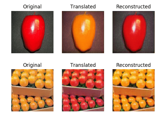
これを実行すると以下のような結果を得られます。
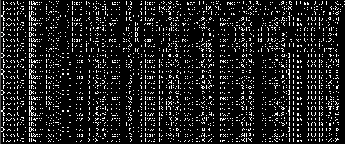
コードの簡単な説明をします。以下の部分で学習を行っています。これが呼び出されるたびにデータローダからデータが読み込まれています。
g_loss = self.combined.train_on_batch([imgs_A, imgs_B],
                                                        [valid, valid,
                                                        imgs_A, imgs_B,
                                                        imgs_A, imgs_B])
                elapsed_time = datetime.datetime.now() - start_time))
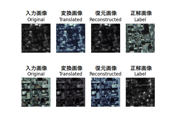
なお、200回ごとにimagesというフォルダに学習過程が保存されていきます。以下に200回と3000回での学習結果を示します。
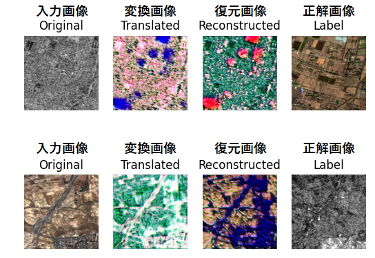
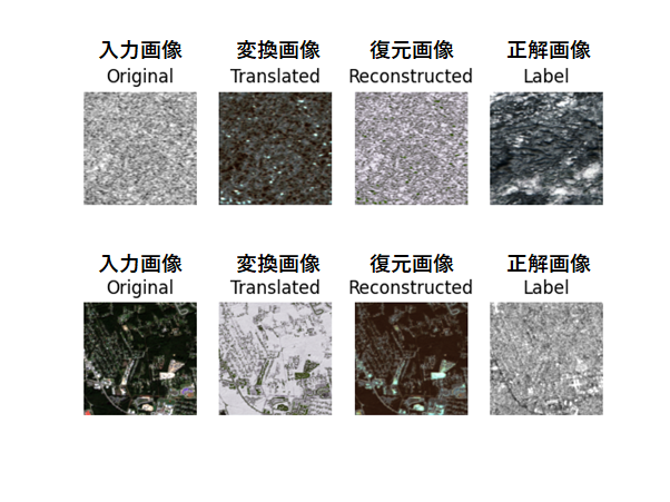
Originalが入力画像、Translatedが変換画像、Reconstructedが変換画像を元に戻した画像、Labelが正解データです。すなわち、Original及びReconstructed、Translated及びLabelの画像が一致していればよいということです。冒頭で説明した数式風に書くと以下のような形式になります。
Original: x ※ウマ
Translated: y := f(x) ※シマウマ
Reconstructed: x := g(f(x)) ※ウマ
Label: y ※シマウマ
上部がSAR→光学→SARに変換した画像です。下部が光学→SAR→光学に変換した画像です。
200回と3000回の学習を比較すると、徐々にSAR画像に近づいていっていることが見て分かります。200回の段階では変換が未熟ですが、3000回目では既にSARのような写りになっています。総当たりで学習しただけで、お互いがペアの学習をしたかのような結果を得られるこの結果は非常に興味深いです。
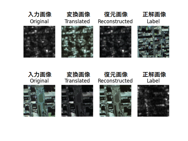
最後に何枚か学習した結果を示します。
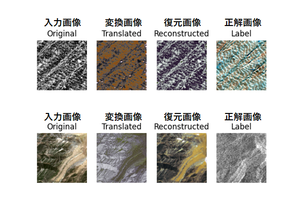
SARから光学画像への変換は、少ない情報量から多い情報量へアップサンプリングする過程があるため、光学からSAR画像程綺麗には変換されませんでした。
※アップサンプリング: 画素数を2倍にする等、元のデータに対して情報量を増加させる処理のこと
4.2. ASNARO-1(光学画像)及びALOS-2(SAR画像)のデータ
では次にこちらのデータセットで実験をしてみます。まず、先ほど作成した2枚の画像を分割してデータセットとして使えるようにします。以下のプログラムをcyclegan.pyを動かしていたフォルダで実行してください。
import cv2
import os
import random
import copy as cp
generation_size = 256
generation_num = 1000
img_a = cv2.imread("SAR.png")
img_b = cv2.imread("OPTICAL.png")
limit_y = img_a.shape[0] - generation_size
output_dir = "./datasets/customsar/"
os.makedirs( output_dir + 'trainA', exist_ok=True)
os.makedirs( output_dir + 'trainB', exist_ok=True)
os.makedirs( output_dir + 'testA', exist_ok=True)
os.makedirs( output_dir + 'testB', exist_ok=True)

for i in range(generation_num):
  offset_y = random.randint(generation_size, img_a.shape[0]) - generation_size
  offset_x = random.randint(generation_size, img_a.shape[1]) - generation_size
  new_a = cp.deepcopy(img_a[offset_y:offset_y+generation_size, offset_x:offset_x+generation_size, :])
  new_b = cp.deepcopy(img_b[offset_y:offset_y+generation_size, offset_x:offset_x+generation_size, :])
  cv2.imwrite(output_dir + "trainA/" + str(i) + ".png", new_a)
  cv2.imwrite(output_dir + "trainB/" + str(i) + ".png", new_b)

split_num = int(img_a.shape[1] / generation_size)
for i in range(split_num):
  offset_y = img_a.shape[0] - generation_size
  offset_x = i * generation_size
  new_a = cp.deepcopy(img_a[offset_y:offset_y+generation_size, offset_x:offset_x+generation_size, :])
  new_b = cp.deepcopy(img_b[offset_y:offset_y+generation_size, offset_x:offset_x+generation_size, :])
  cv2.imwrite(output_dir + "testA/" + str(i) + ".png", new_a)
  cv2.imwrite(output_dir + "testB/" + str(i) + ".png", new_b)
これを実行すると./datasets/customsar/のフォルダ配下に「trainA, trainB, testA, testB」といったフォルダが生成され、各ドメインの画像が別けられます。AがSARでBが光学ドメインとなっています。
では、次にcyclegan.pyを以下のように変更して実行しましょう。
変更前 self.dataset_name = ‘sar’
変更後 self.dataset_name = ‘customsar’
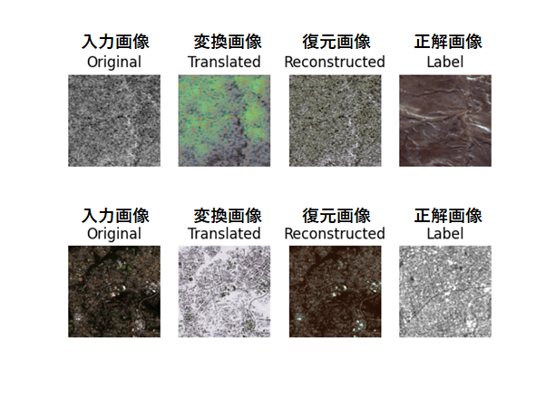
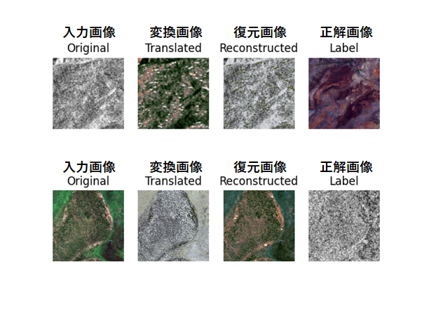
以下のような実行結果が得られます。
一方のデータセットほど綺麗に変換はされませんでしたが、解像度が粗い割には、近いような画像が生成されているのではないでしょうか。SARが反射しそうなところは白く残り、他は暗くなるような学習をしています。
Sentinel-1/2のペアもASNARO-1/ALOS-2のペアも、どちらのデータセットも画像をランダム化して学習しているので、ASNARO-1/ALOS-2のデータセットもSAR側の解像度が高ければ一方のデータセットと同じくらい綺麗に変換出来ていたのではないかと思います。
では、参考までにいくつか実行結果を示します。
5. 教師あり学習(pix2pix)による光学↔SAR画像変換
次に教師あり学習だとどうなるか試してみましょう。CycleGAN同様に、実装は(https://github.com/eriklindernoren/Keras-GAN/tree/master/pix2pix)を参考に実装していきました。主にバージョン互換、データローダ等について変更が加わっています。データセットはcycleganで用いたものをそのまま流用できるので、新たに作業フォルダを作成し、datasetsのみcycleganからコピーして下さい。新たに作成したフォルダはルートディレクトリとして扱います。流れに沿ってプログラムを実行していけば以下のようなフォルダ構成になるはずです。
root
|- pix2pix.py
|- data_loader_py
|- datasets
| |- sat
| |-testA
| | |- file...
| |-testB
| | |- file...
| |-trainA
| | |- file...
| |-trainB
| |- file...
|- images
|- sar
|- file…
5.1. 高品質な光学及びSARのペア画像(Sentinel-1, 2)
まずはデータ読み込み部分のデータローダを示します。data_loader.pyという名前で保存してください。
import scipy
from glob import glob
import numpy as np
import matplotlib.pyplot as plt

class DataLoader():
    def __init__(self, dataset_name, img_res=(128, 128)):
        self.dataset_name = dataset_name
        self.img_res = img_res

    def load_data(self, batch_size=1, is_testing=False):
        data_type = "train" if not is_testing else "test"
        path = glob('./datasets/%s/%s/*' % (self.dataset_name, data_type))

        batch_images = np.random.choice(path, size=batch_size)

        imgs_A = []
        imgs_B = []
        for img_path in batch_images:
            img = self.imread(img_path)

            h, w, _ = img.shape
            _w = int(w/2)
            img_A, img_B = img[:, :_w, :], img[:, _w:, :]

            img_A = scipy.misc.imresize(img_A, self.img_res)
            img_B = scipy.misc.imresize(img_B, self.img_res)

            # If training => do random flip
            if not is_testing and np.random.random()  0.5:
                        img_A = np.fliplr(img_A)
                        img_B = np.fliplr(img_B)

                imgs_A.append(img_A)
                imgs_B.append(img_B)

            imgs_A = np.array(imgs_A)/127.5 - 1.
            imgs_B = np.array(imgs_B)/127.5 - 1.

            yield imgs_A, imgs_B

    def load_data_with_label_batch(self, domain, batch_size=1, is_testing=False):
        data_type = "train%s" % domain if not is_testing else "test%s" % domain
        path = glob('./datasets/%s/%s/*' % (self.dataset_name, data_type))
        batch_images = np.random.choice(path, size=batch_size)
        imgs = []
        lbls = []
        for img_path in batch_images:
            img = self.imread(img_path)
            # lbl path
            if "A/" in img_path:
              lbl_path = img_path.replace('s1_', 's2_')
              lbl_path = lbl_path.replace('A/', 'B/')
            else:
              lbl_path = img_path.replace('s2_', 's1_')
              lbl_path = lbl_path.replace('B/', 'A/')
            lbl = self.imread(lbl_path)

            if not is_testing:
                img = scipy.misc.imresize(img, self.img_res)
                lbl = scipy.misc.imresize(lbl, self.img_res)

                if np.random.random() > 0.5:
                    img = np.fliplr(img)
                    lbl = np.fliplr(lbl)
            else:
                img = scipy.misc.imresize(img, self.img_res)
                lbl = scipy.misc.imresize(lbl, self.img_res)
            imgs.append(img)
            lbls.append(lbl)
        imgs = np.array(imgs)/127.5 - 1.
        lbls = np.array(lbls)/127.5 - 1.
        return imgs, lbls


    def imread(self, path):
        return scipy.misc.imread(path, mode='RGB').astype(np.float)
次にpix2pix本体のプログラムです。pix2pix.pyという名前で保存しましょう。
from __future__ import print_function, division
import scipy
from keras.datasets import mnist
from keras_contrib.layers.normalization.instancenormalization import InstanceNormalization
from keras.layers import Input, Dense, Reshape, Flatten, Dropout, Concatenate
from keras.layers import BatchNormalization, Activation, ZeroPadding2D
from keras.layers.advanced_activations import LeakyReLU
from keras.layers.convolutional import UpSampling2D, Conv2D
from keras.models import Sequential, Model
from tensorflow.keras.optimizers import Adam
import datetime
import matplotlib.pyplot as plt
import sys
from data_loader import DataLoader
import numpy as np
import os
import matplotlib as mpl
mpl.use('Agg')
import matplotlib.pyplot as plt

class Pix2Pix():
    def __init__(self):
        # Input shape
        self.img_rows = 256
        self.img_cols = 256
        self.channels = 3
        self.img_shape = (self.img_rows, self.img_cols, self.channels)

        # Configure data loader
        self.dataset_name = 'sar'
        self.data_loader = DataLoader(dataset_name=self.dataset_name,
                                      img_res=(self.img_rows, self.img_cols))


        # Calculate output shape of D (PatchGAN)
        patch = int(self.img_rows / 2**4)
        self.disc_patch = (patch, patch, 1)

        # Number of filters in the first layer of G and D
        self.gf = 64
        self.df = 64

        optimizer = Adam(0.0002, 0.5)

        # Build and compile the discriminator
        self.discriminator = self.build_discriminator()
        self.discriminator.compile(loss='mse',
            optimizer=optimizer,
            metrics=['accuracy'])

        #-------------------------
        # Construct Computational
        #   Graph of Generator
        #-------------------------

        # Build the generator
        self.generator = self.build_generator()

        # Input images and their conditioning images
        img_A = Input(shape=self.img_shape)
        img_B = Input(shape=self.img_shape)

        # By conditioning on B generate a fake version of A
        fake_A = self.generator(img_B)

        # For the combined model we will only train the generator
        self.discriminator.trainable = False

        # Discriminators determines validity of translated images / condition pairs
        valid = self.discriminator([fake_A, img_B])

        self.combined = Model(inputs=[img_A, img_B], outputs=[valid, fake_A])
        self.combined.compile(loss=['mse', 'mae'],
                              loss_weights=[1, 100],
                              optimizer=optimizer)

    def build_generator(self):
        """U-Net Generator"""

        def conv2d(layer_input, filters, f_size=4, bn=True):
            """Layers used during downsampling"""
            d = Conv2D(filters, kernel_size=f_size, strides=2, padding='same')(layer_input)
            d = LeakyReLU(alpha=0.2)(d)
            if bn:
                d = BatchNormalization(momentum=0.8)(d)
            return d

        def deconv2d(layer_input, skip_input, filters, f_size=4, dropout_rate=0):
            """Layers used during upsampling"""
            u = UpSampling2D(size=2)(layer_input)
            u = Conv2D(filters, kernel_size=f_size, strides=1, padding='same', activation='relu')(u)
            if dropout_rate:
                u = Dropout(dropout_rate)(u)
            u = BatchNormalization(momentum=0.8)(u)
            u = Concatenate()([u, skip_input])
            return u

        # Image input
        d0 = Input(shape=self.img_shape)

        # Downsampling
        d1 = conv2d(d0, self.gf, bn=False)
        d2 = conv2d(d1, self.gf*2)
        d3 = conv2d(d2, self.gf*4)
        d4 = conv2d(d3, self.gf*8)
        d5 = conv2d(d4, self.gf*8)
        d6 = conv2d(d5, self.gf*8)
        d7 = conv2d(d6, self.gf*8)

        # Upsampling
        u1 = deconv2d(d7, d6, self.gf*8)
        u2 = deconv2d(u1, d5, self.gf*8)
        u3 = deconv2d(u2, d4, self.gf*8)
        u4 = deconv2d(u3, d3, self.gf*4)
        u5 = deconv2d(u4, d2, self.gf*2)
        u6 = deconv2d(u5, d1, self.gf)

        u7 = UpSampling2D(size=2)(u6)
        output_img = Conv2D(self.channels, kernel_size=4, strides=1, padding='same', activation='tanh')(u7)

        return Model(d0, output_img)

    def build_discriminator(self):

        def d_layer(layer_input, filters, f_size=4, bn=True):
            """Discriminator layer"""
            d = Conv2D(filters, kernel_size=f_size, strides=2, padding='same')(layer_input)
            d = LeakyReLU(alpha=0.2)(d)
            if bn:
                d = BatchNormalization(momentum=0.8)(d)
            return d

        img_A = Input(shape=self.img_shape)
        img_B = Input(shape=self.img_shape)

        # Concatenate image and conditioning image by channels to produce input
        combined_imgs = Concatenate(axis=-1)([img_A, img_B])

        d1 = d_layer(combined_imgs, self.df, bn=False)
        d2 = d_layer(d1, self.df*2)
        d3 = d_layer(d2, self.df*4)
        d4 = d_layer(d3, self.df*8)

        validity = Conv2D(1, kernel_size=4, strides=1, padding='same')(d4)

        return Model([img_A, img_B], validity)

    def train(self, epochs, batch_size=1, sample_interval=50):

        start_time = datetime.datetime.now()

        # Adversarial loss ground truths
        valid = np.ones((batch_size,) + self.disc_patch)
        fake = np.zeros((batch_size,) + self.disc_patch)

        for epoch in range(epochs):
            for batch_i, (imgs_A, imgs_B) in enumerate(self.data_loader.load_batch(domain="A", batch_size=batch_size)):

                # ---------------------
                #  Train Discriminator
                # ---------------------

                # Condition on B and generate a translated version
                fake_A = self.generator.predict(imgs_B)

                # Train the discriminators (original images = real / generated = Fake)
                d_loss_real = self.discriminator.train_on_batch([imgs_A, imgs_B], valid)
                d_loss_fake = self.discriminator.train_on_batch([fake_A, imgs_B], fake)
                d_loss = 0.5 * np.add(d_loss_real, d_loss_fake)

                # -----------------
                #  Train Generator
                # -----------------

                # Train the generators
                g_loss = self.combined.train_on_batch([imgs_A, imgs_B], [valid, imgs_A])

                elapsed_time = datetime.datetime.now() - start_time
                # Plot the progress
                print ("[Epoch %d/%d] [Batch %d/%d] [D loss: %f, acc: %3d%%] [G loss: %f] time: %s" % (epoch, epochs,
                                                                        batch_i, self.data_loader.n_batches,
                                                                        d_loss[0], 100*d_loss[1],
                                                                        g_loss[0],
                                                                        elapsed_time))

                # If at save interval => save generated image samples
                if batch_i % sample_interval == 0:
                    self.sample_images(epoch, batch_i)

    def sample_images(self, epoch, batch_i):
        os.makedirs('images/%s' % self.dataset_name, exist_ok=True)
        r, c = 3, 3

        imgs_A, imgs_B = self.data_loader.load_data_with_label_batch(domain="A", batch_size=3, is_testing=True)
        fake_A = self.generator.predict(imgs_B)

        gen_imgs = np.concatenate([imgs_B, fake_A, imgs_A])

        # Rescale images 0 - 1
        gen_imgs = 0.5 * gen_imgs + 0.5

        titles = ['Condition', 'Generated', 'Original']
        fig, axs = plt.subplots(r, c)
        cnt = 0
        for i in range(r):
            for j in range(c):
                axs[i,j].imshow(gen_imgs[cnt])
                axs[i, j].set_title(titles[i])
                axs[i,j].axis('off')
                cnt += 1
        fig.savefig("images/%s/%d_%d.png" % (self.dataset_name, epoch, batch_i))
        plt.close()


if __name__ == '__main__':
    gan = Pix2Pix()
    gan.train(epochs=200, batch_size=3, sample_interval=200)
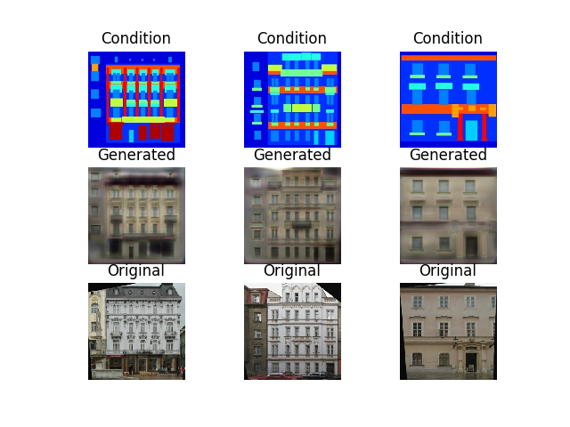
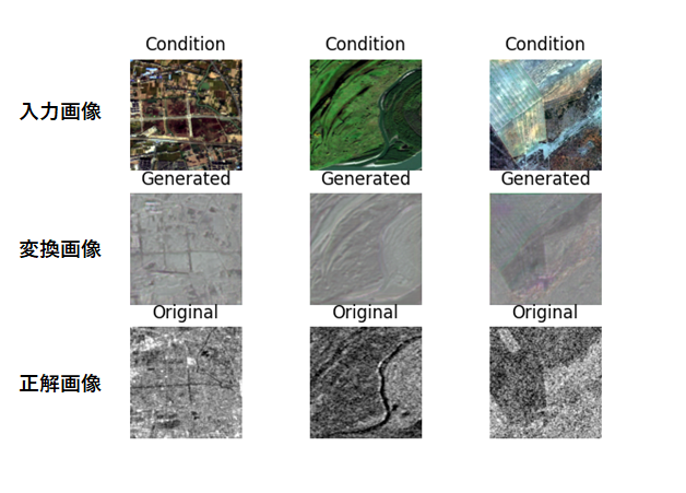
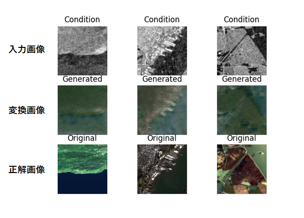
これを実行すると以下のような結果が得られます。
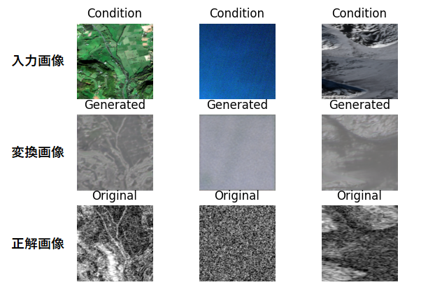
Conditionが入力画像(光学画像)、Generatedが変換画像(SAR画像)、Originalが答え(SAR画像)です。つまるところ、GeneratedとOriginalが一致していればよいわけです。
感覚的には教師あり学習の方が高精度な画像を出力してくると思いましたが、教師なし学習と大差ないように感じます。他の結果も参考までにいくつか示します。
なお、逆向きにSAR→光学画像の変換を学習させるには以下のように変更して学習させてください。
変更前 for batch_i, (imgs_A, imgs_B) in enumerate(self.data_loader.load_batch(domain=”A”, batch_size=batch_size)):
変更後 for batch_i, (imgs_A, imgs_B) in enumerate(self.data_loader.load_batch(domain=”B”, batch_size=batch_size)):
変更前 imgs_A, imgs_B = self.data_loader.load_data_with_label_batch(domain=”A”, batch_size=3, is_testing=True)
変更後 imgs_A, imgs_B = self.data_loader.load_data_with_label_batch(domain=”B”, batch_size=3, is_testing=True)
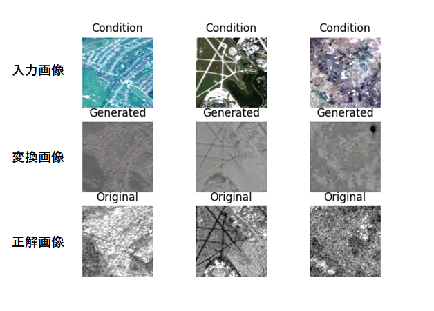
実行すると以下のような結果を得られます。
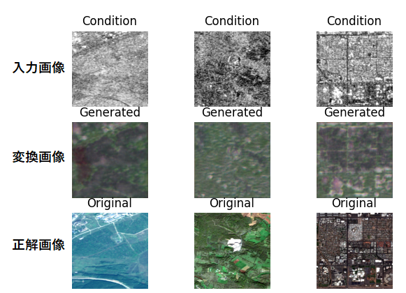
光学→SARよりもSAR→光学のほうが得意なように見受けられます。情報量は光学の方が多そうなので興味深いですね。 しかし、色合いを間違えてしまうことはよくあるようです。以下に他の例も示します。
5.2. ASNARO-1(光学画像)及びALOS-2(SAR画像)のデータ
教師なし学習の方と同様に以下の部分のみを変更して実行してください。
変更前 self.dataset_name = ‘sar’
変更後 self.dataset_name = ‘customsar’
※光学→SARの変換をするため、前述で変更したソースコードのdomainを元に戻すようにして下さい
以下のような結果が得られます。
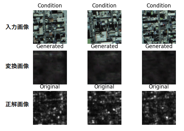
こちらは高品質なペア画像(解像度、仕様、観測時期が同じ等)ではないため、結果もイマイチなものになってしまいました。他の結果もほとんど真っ暗になってしまいました。こちらについてはCycleGANを用いた教師なし学習の方が上手く動いていますね。もちろん、学習度合いに応じて結果は変わるのでぜひ皆様も試してみて下さい。
では、次にSAR→光学も試してみましょう。やり方はもう一方のデータセットでの方法と同じで、pix2pix.pyのソースコードを以下のように変更します。
変更前 for batch_i, (imgs_A, imgs_B) in enumerate(self.data_loader.load_batch(domain=”A”, batch_size=batch_size)):
変更後
for batch_i, (imgs_A, imgs_B) in enumerate(self.data_loader.load_batch(domain=”B”, batch_size=batch_size)):
変更前 imgs_A, imgs_B = self.data_loader.load_data_with_label_batch(domain=”A”, batch_size=3, is_testing=True)
変更後 imgs_A, imgs_B = self.data_loader.load_data_with_label_batch(domain=”B”, batch_size=3, is_testing=True)
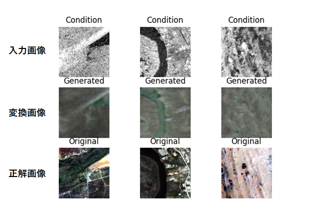
これを実行すると以下のような結果を得られます。
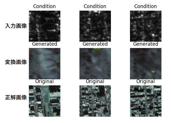
こちらについても殆ど変換が上手く出来ていません。他の結果も殆どがボヤッとした映りになってしまっています。教師あり学習は、やはりペア画像の品質にかなり左右されるということでしょうか。
長くなりましたが、ここまででASNARO-1及びALOS-2並びにSentinel-1及びSentinel-2の2種類のデータセットを用いて、教師なし学習(cyclegan)及び教師あり学習(pix2pix)で光学及びSAR画像間の相互変換を試しました。最後のまとめでは、これ等で得られた結果を基に比較を、行い向き不向きのマトリクス表を作成したいと思います。
6. まとめ
本稿では以下のことについて挑戦しました。
・ASNARO-1(光学画像)及びALOS-2(SAR画像)のデータを雑に集めて、光学↔SAR画像の相互変換を行う
・高品質な光学及びSARのペア画像(Sentinel-1, 2)を用いて光学↔SAR画像変換を行う
・光学↔SAR画像変換は教師なし(CycleGAN)、教師あり(Pix2Pix)学習の両方で行い、その違いを比較する
データセット2つに対して2つの手法を試したので、結果は4つ得られました。それでは、4つの結果を比較してみたいと思います。
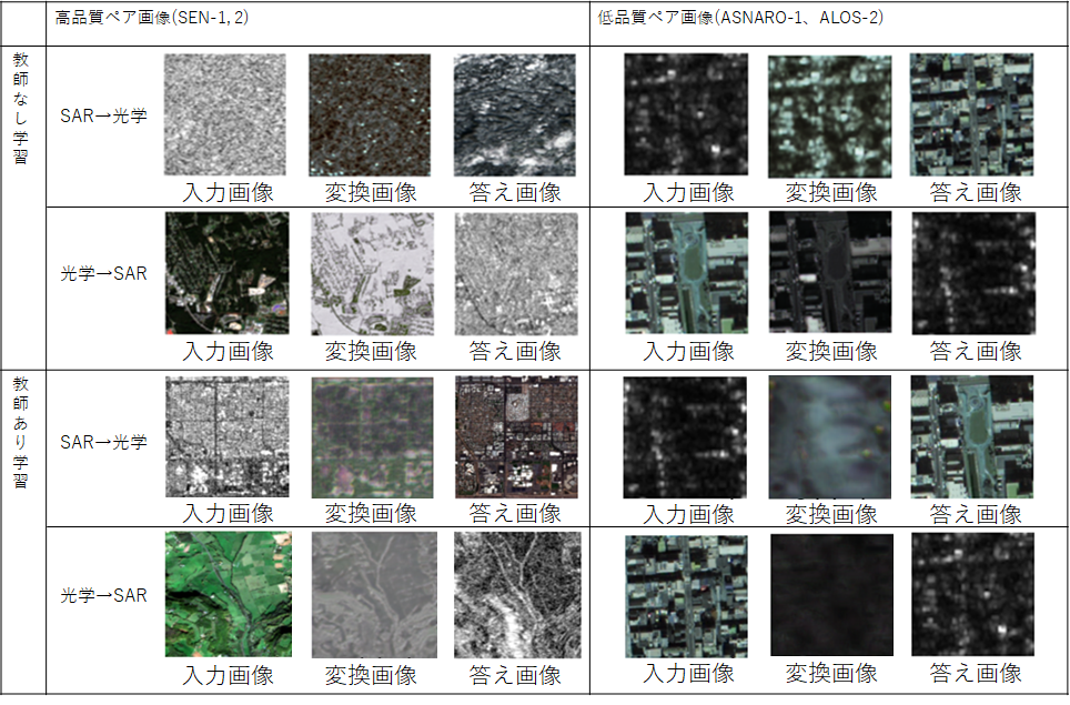
高品質ペア画像は教師なしでも教師ありでも、それなりに変換されていることが確認できます。低品質ペアに限っては教師なし学習では、それなりに変換されているものの、教師あり学習では全く上手く変換できていません。これをマトリクス表でまとめると以下のようになります。
| 高品質ペア画像(Sentinel-1, 2) | 低品質ペア画像(ASNARO-1、ALOS-2) | |
| 教師なし学習 | 〇 | 〇 |
| 教師あり学習 | 〇 | × |
このことから、高品質なペア画像が揃えられない場合は教師なし学習のCycleGANが使えるということが分かりました。一方で高品質なペア画像が揃えられる場合は、教師なし学習でも教師あり学習でも大きな違いがないということが分かりました。
教師なし学習を用いることで、高品質でない不揃いなペア画像からでもSAR画像を生成出来ることが分かりました。この技術を使うことで「ある光学衛星にSARを搭載したらどのように写る」のかであったり、「あるSAR衛星に光学を搭載したらどのように写る」のかを試すことができます。また、そもそもSARで一度も観測されたことない物体がどのように写るのかシミュレーションすることもできます。この技術は非常に幅広く応用が利くため、皆様のアイディアに生かしてみては如何でしょうか。
以上ありがとうございました。